Project 2: Fun with Filters and Frequencies!
Overview
In this project, I explored image filtering, edge detection, and multi-resolution blending. The assignment was divided into two main parts:
- Part 1: Fun with Filters — convolution, finite differences, and derivative of Gaussian.
- Part 2: Fun with Frequencies — sharpening, hybrid images, Gaussian/Laplacian stacks, and multi-resolution blending (the famous Oraple!).
Part 1: Filters and Edges
Part 1.1: Convolutions from Scratch!
In this section, I implemented convolution in three ways: first using four nested loops, then
with two nested loops, and finally by comparing against the built-in
scipy.signal.convolve2d.
All implementations supported zero-padding to handle boundaries and the runtime for the four-loop version is O(H * W * KH * KW), (Height * Width * Kernel Height * Kernel Width), while the runtime for the two-loop is only O(H*W) since it's vectorized.
To test, I created a 9×9 box filter and applied it to a grayscale image of Lebron and Draymond Green.
I also convolved the image with finite difference operators
Dx and Dy.
Below is my main convolution function, which calls either the two-loop or four-loop implementation:
            def convolve_2D(image, kernel, pad_width = 0, mul_type="two_loop"):

            image = np.array(image, dtype=np.float32)
            kernel = np.array(kernel, dtype=np.float32)

            # * Here is the padding part of the code, for loops that insert 0s according to pad_width
            # * numpy doesn't allow array size changes so a new array has to be created

            def _pad_image(image, pad_width):
                padded_image = np.full((image.shape[0] + 2 *pad_width, image.shape[1] + 2 * pad_width), 0, dtype=np.float32)

                for row in range(image.shape[0]):
                    for col in range(image.shape[1]):
                        padded_image[row + pad_width][col + pad_width] = image[row][col]

                return padded_image


        # * _pad_image is a helper function we can pull out of the bag here only if needed

            if(pad_width):
                image = _pad_image(image, pad_width)

                print(image)

        # * After creating the padded image, we can create the holder for the reusult
        # * The formula for the shape is padded_image_dim - kernel_dim + 1

            result = np.full((image.shape[0] - kernel.shape[0] + 1, image.shape[1] - kernel.shape[1] + 1), 0, dtype=np.float32)


        # * Since this is a convolution, we should flip the kernel

            kernel = np.flip(kernel)

        # * Now we have both the flipped image and the rotated kernel, so we should be able to multiply and add


        # * This is a four for-loop convolution implementation
            def element_wise_dot_four(image, kernel):
                for slide_right_num in range(image.shape[0] - kernel.shape[0] + 1):
                    for slide_down_num in range(image.shape[1] - kernel.shape[1] + 1):
                        addition_holder = 0
                        for row in range(kernel.shape[0]):
                            for col in range(kernel.shape[1]):
                                addition_holder += kernel[row][col] * image[row + slide_right_num][col + slide_down_num]

                        result[slide_right_num][slide_down_num] = addition_holder
                        addition_holder = 0

                return result

        # * This is a two for-loop convolution implementation

            def element_wise_dot_two(image, kernel):
                for row in range(result.shape[0]):
                    for col in range(result.shape[1]):
                        window = image[row:row+kernel.shape[0], col:col+kernel.shape[1]]

                        result[row][col] = np.sum(window * kernel)

                return result


            if mul_type == "two_loop":
                result = element_wise_dot_two(image, kernel)
            else:
                result = element_wise_dot_four(image, kernel)

            return result
These are the kernel implementations:
            box_filter = 1/9 * np.full((3,3), 1, dtype=np.float32)

            my_convolved_image = convolve_2D(gray, box_filter, pad_width=0)

            builtin_convolved_image = scipy.signal.convolve2d(gray, box_filter, mode="valid")

            '''
            '''
            # * Now I'm going to use these as kernels instead

            dx = np.array([[1, 0, -1]])
            dy = np.array([[1],[0],[-1]])

            my_dx_image = convolve_2D(gray, dx, pad_width=0)

            my_dy_image = convolve_2D(gray, dy, pad_width=0)

            builtin_dx_image = scipy.signal.convolve2d(gray, dx, mode="valid")
            builtin_dy_image = scipy.signal.convolve2d(gray, dy, mode="valid")

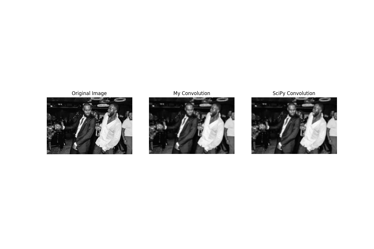
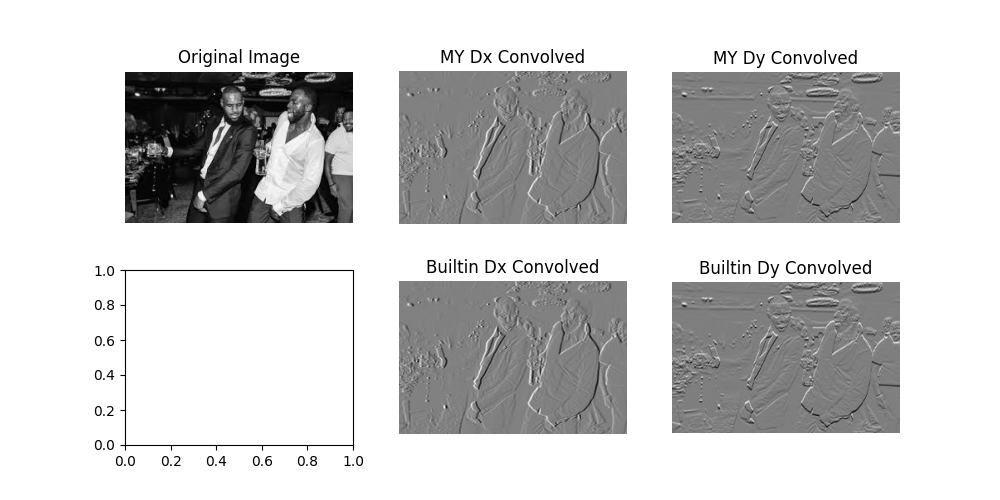
The results from my implementation matched those from scipy.signal.convolve2d.
Runtime was significantly faster using the built-in function, but the custom code
helped build intuition for how convolutions operate at the pixel level.
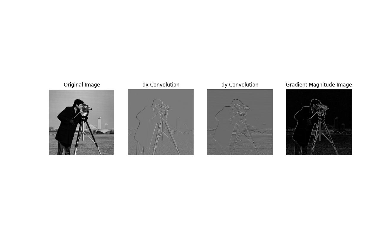
Part 1.2: Finite Difference Operator
In this section, I applied the finite difference operators
Dx and Dy to the
Cameraman image to compute horizontal and vertical image gradients.
These operators highlight edges by capturing intensity changes along the x and y directions.
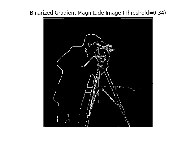
I then combined them to calculate the gradient magnitude, which emphasizes overall edge strength.
Finally, I binarized the gradient magnitude using a threshold value (0.34) to produce a clear edge map.
This demonstrates how simple derivative filters can be used for edge detection.
Part 1.3: Derivative of Gaussian (DoG) Filter
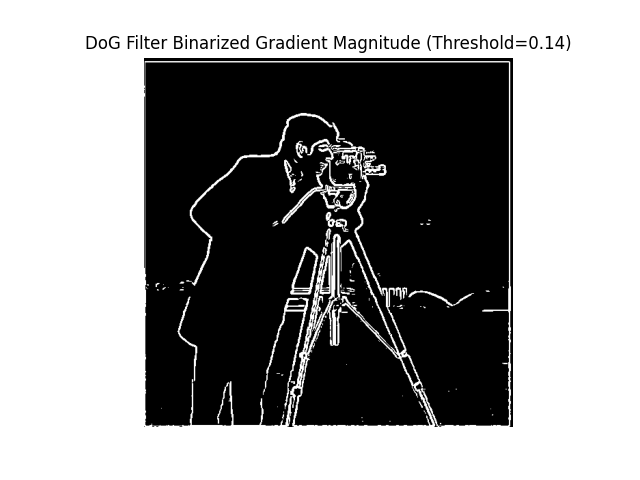
In this part, I reduced noise by first smoothing the image with a Gaussian filter before
applying the finite difference operators. This produced cleaner edge maps compared to
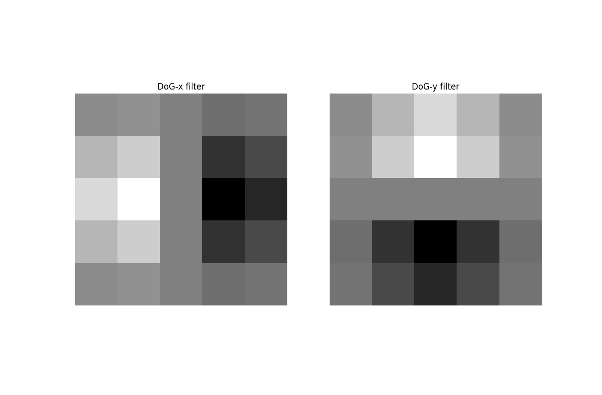
the raw derivatives from Part 1.2. I also constructed derivative of Gaussian (DoG) filters
by convolving the Gaussian kernel with Dx and Dy.
Using these DoG filters directly gives the same result as applying Gaussian smoothing first,
then taking derivatives. Compare the DoG Filter Binarized Gradient Magnitute (threshold = 0.14)
to the one above and notice that it looks better.
Part 2: Fun with Frequencies
Part 2.1: Image Sharpening
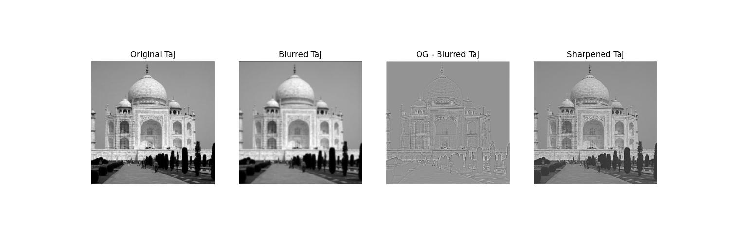
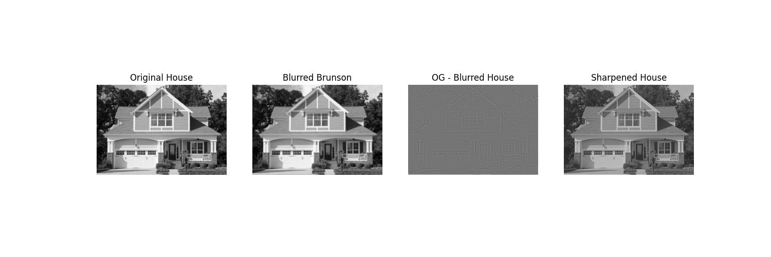
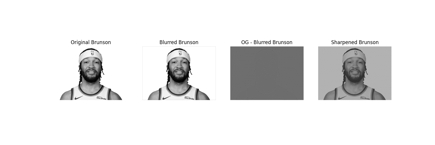
In this part, I implemented image sharpening using the unsharp masking technique. First, I applied a Gaussian filter to the Taj Mahal image to extract its low-frequency components (the blurred version). Subtracting this blurred image from the original left me with the high-frequency details such as edges and fine textures. By adding these high-frequency details back to the original image, I produced a sharpened result that enhances edges and makes the image appear crisper. This demonstrates how unsharp masking works by amplifying high-frequency content while preserving the overall structure of the image.
I similarly applied the procedure below to an image of a house. You can see that it does look sharper, but a little darkly glazed.
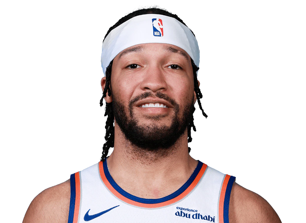
Notice here that I also applied the same to an already high-res image of Jalen Brunson. You can see that the result is not nearly as good as the original.
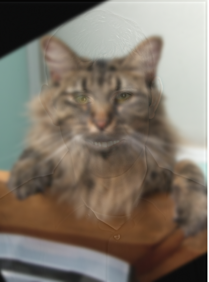
Part 2.2: Hybrid Images
In this part, I created three hybrid images: the classic Derek + Nutmeg pair (as required) and two
additional hybrids of my own choosing. For the Derek + Nutmeg hybrid, I carefully walked through the
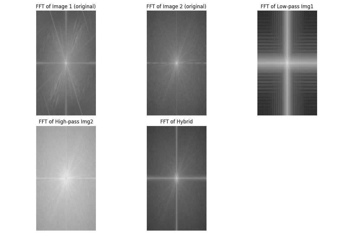
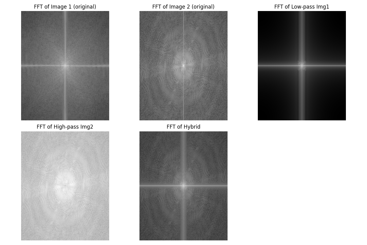
entire pipeline: starting with the original, aligned input images, computing and visualizing
their Fourier transforms, generating the low-pass filtered result for one image, and extracting
the high-pass component of the other. A key step here was the cutoff frequency choice, which I
set by selecting the Gaussian blur parameter (σ = 6 with a 31×31 kernel). This parameter
determined what counted as “low-frequency” structure versus “high-frequency” detail. Choosing too small of a
cutoff left both images overly sharp and hard to separate, while too large of a cutoff lost important
structure. With this setting, the hybrid image clearly looks like Derek up close (high frequencies dominate)
but transitions to Nutmeg from afar (low frequencies dominate). I also included the final hybrid image
and its frequency spectrum visualization to confirm that the low- and high-frequency information were
separated correctly.
For my two additional hybrids, I presented the original input images alongside the final blended
results. These demonstrate how the same technique generalizes beyond the canonical example, and highlight how
alignment, filter size, and cutoff frequency choices influence the outcome of the hybrid. Across all three
examples, this process shows how Gaussian blurs and frequency-domain reasoning can be combined to generate
perceptually interesting images that depend on viewing distance.
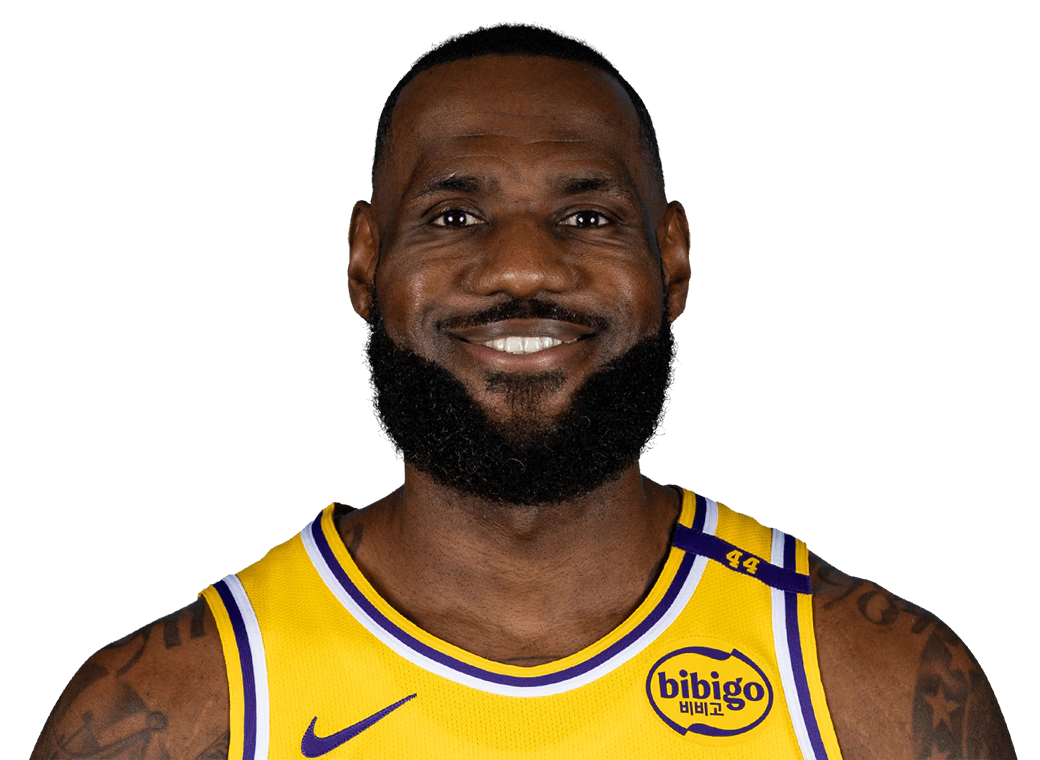
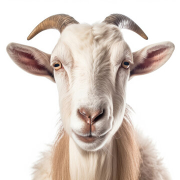
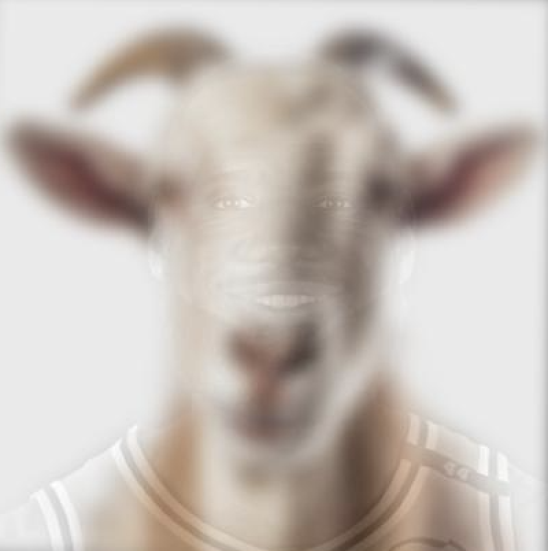
Below, I repeat the hybrid image process using a picture of LeBron and a goat:
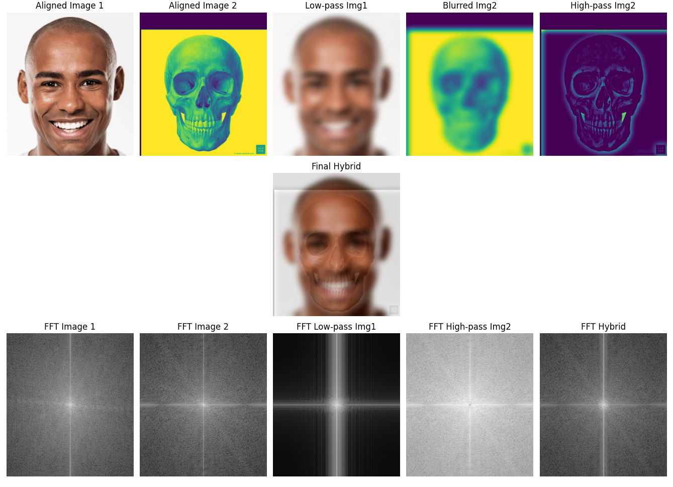
Below, I repeat the hybrid image process using a picture of a face and a skull:
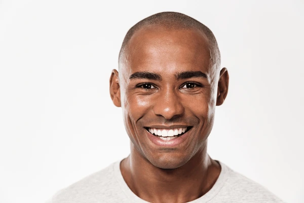
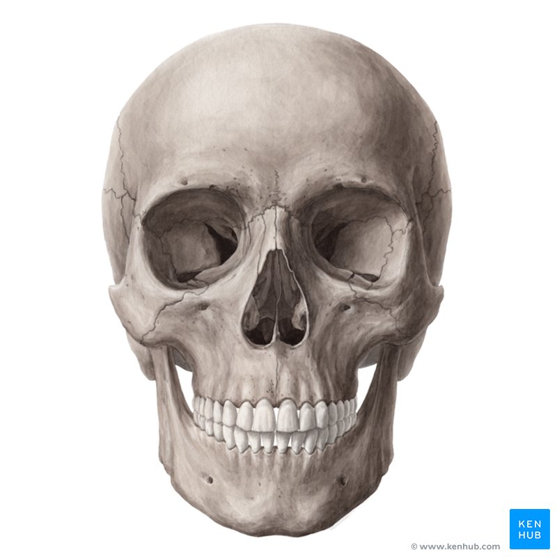
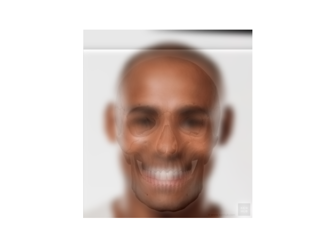
Now, here's a comprehensive figure including the alignment and everything else. I believe the skull is a weird color because normalization is applied before displaying the hybrid, so it all looks fine in the end. Pretty cool looking though, maybe I should've kept it un-normalized.
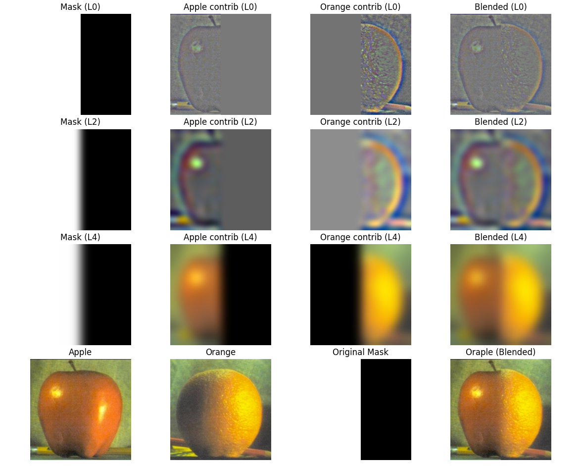
Part 2.3: Gaussian and Laplacian Stacks
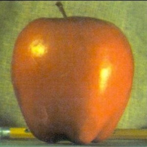
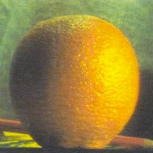
In this part, I recreated the famous "Oraple" figure by blending an apple and an orange using
Gaussian and Laplacian stacks. To do this, I reused and extended some of my code from Project 1,
where I had already implemented Gaussian pyramids and convolution from scratch. I modified the
functions so they would support RGB images and increased the kernel size to produce smoother
results suitable for multi-resolution blending. The process involved building Gaussian stacks for
the input images and a binary mask, constructing Laplacian stacks by subtracting adjacent Gaussian
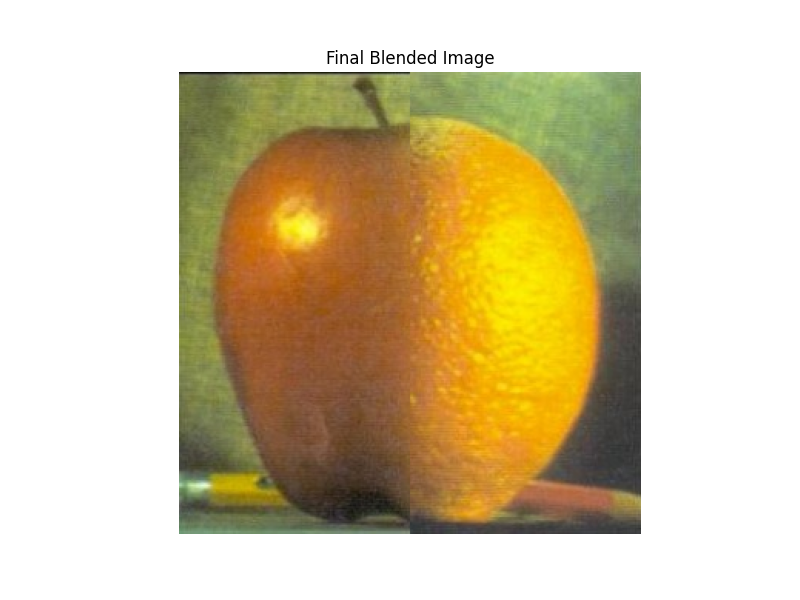
levels, and then blending contributions from both images level by level. Finally, I collapsed the
blended Laplacian stack to form the hybrid "Oraple."
Using these functions, I was able to recreate figure 3.42 in the Szeliski book
Part 2.4: Multiresolution Blending (The Oraple!)
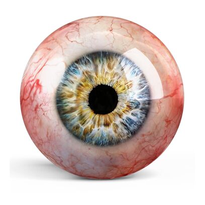
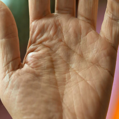
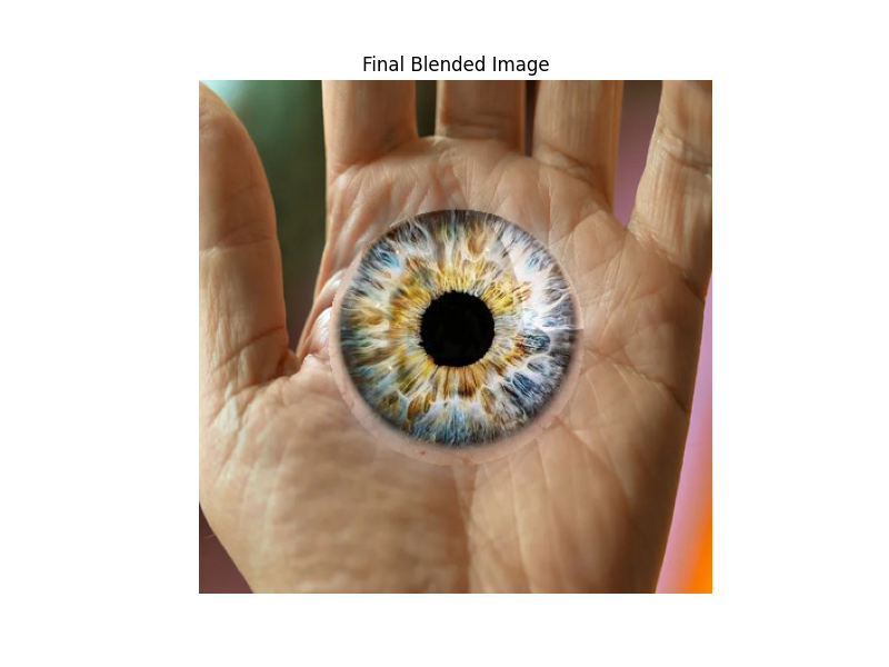
In this final part, I extended the multi-resolution blending technique from Part 2.3 by experimenting with different mask shapes. Instead of only using a vertical split mask (square), I also created a circular mask to blend images more naturally around a central region. This allowed me to produce more interesting composite images where the transition between the two inputs is smoother and less obvious, which you can see for the eye-hand image. The implementation reused my Gaussian and Laplacian stack code from earlier parts, but generalized it so that any mask shape can be applied for blending. This demonstrates the flexibility of stack-based blending beyond just the traditional "Oraple" example. However, since we used a stack instead of a pyramid, there's no blending at L0, which makes those details appear somewhat stark, as seen below.
Here's an example of me using my circular mask for a cool hand-eye.
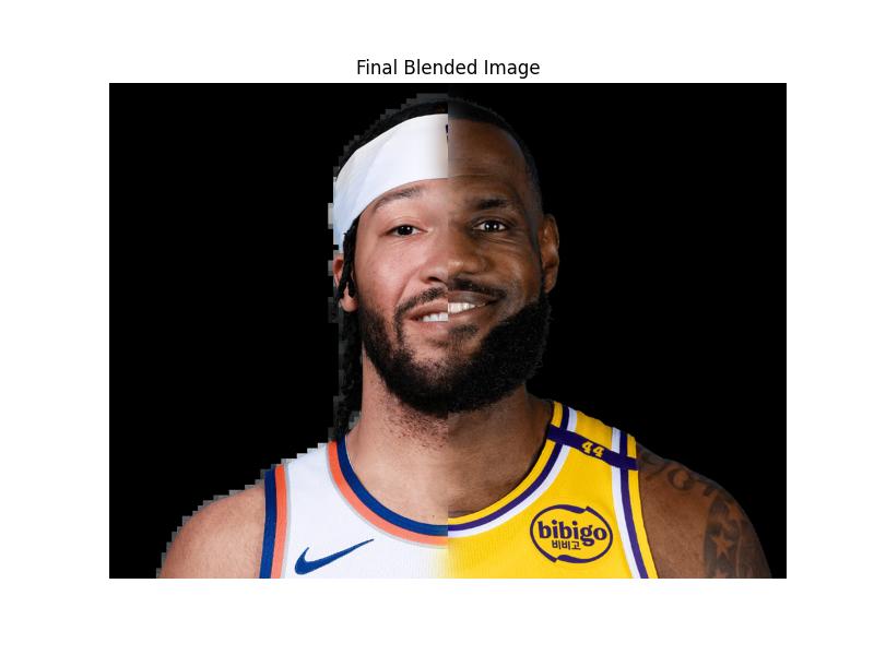
I also wanted to try using the square mask to combine jalen brunson and lebron.
What I Learned
The most important thing I learned was how frequency analysis reveals structure that’s invisible in raw pixel space. From edge detection to hybrid images and blending, frequency decomposition makes image manipulation both efficient and perceptually convincing. Also, the importance of the lowest level of detail during the multiresolution blending section was really interesting. Also, this took pretty long, so I didn't have time to do bells and whistles unfortunately.