CS180 Project 4 — Neural Radiance Fields

Project 4: Neural Radiance Fields (NeRF)

Overview

The goal of this project was to implement Neural Radiance Fields (NeRF) from scratch. I started by calibrating my own camera using ArUco markers, fitting a simple neural network to a 2D image, and finally implementing a full volumetric rendering pipeline to reconstruct 3D scenes from 2D images. This writeup details each part of the project along with results and challenges encountered.

Part 0 — Camera Calibration & Data Capture

Before training the NeRF, I needed to capture a dataset with known camera poses. I used a grid of ArUco markers to solve the Perspective-n-Point (PnP) problem.

0.1: Camera Intrinsics Calibration

I captured 30-50 calibration images of ArUco tags from various angles and distances. Using cv2.detectMarkers() and cv2.calibrateCamera(), I computed the camera intrinsic matrix K and distortion coefficients that minimize reprojection error between observed 2D points and known 3D marker corners.

TAG_SIZE = 0.06 meters

Calibration RMS Error: 2.07

Camera Matrix K and distortion coefficients saved to camera_params.npz

0.2: Object Scan Capture

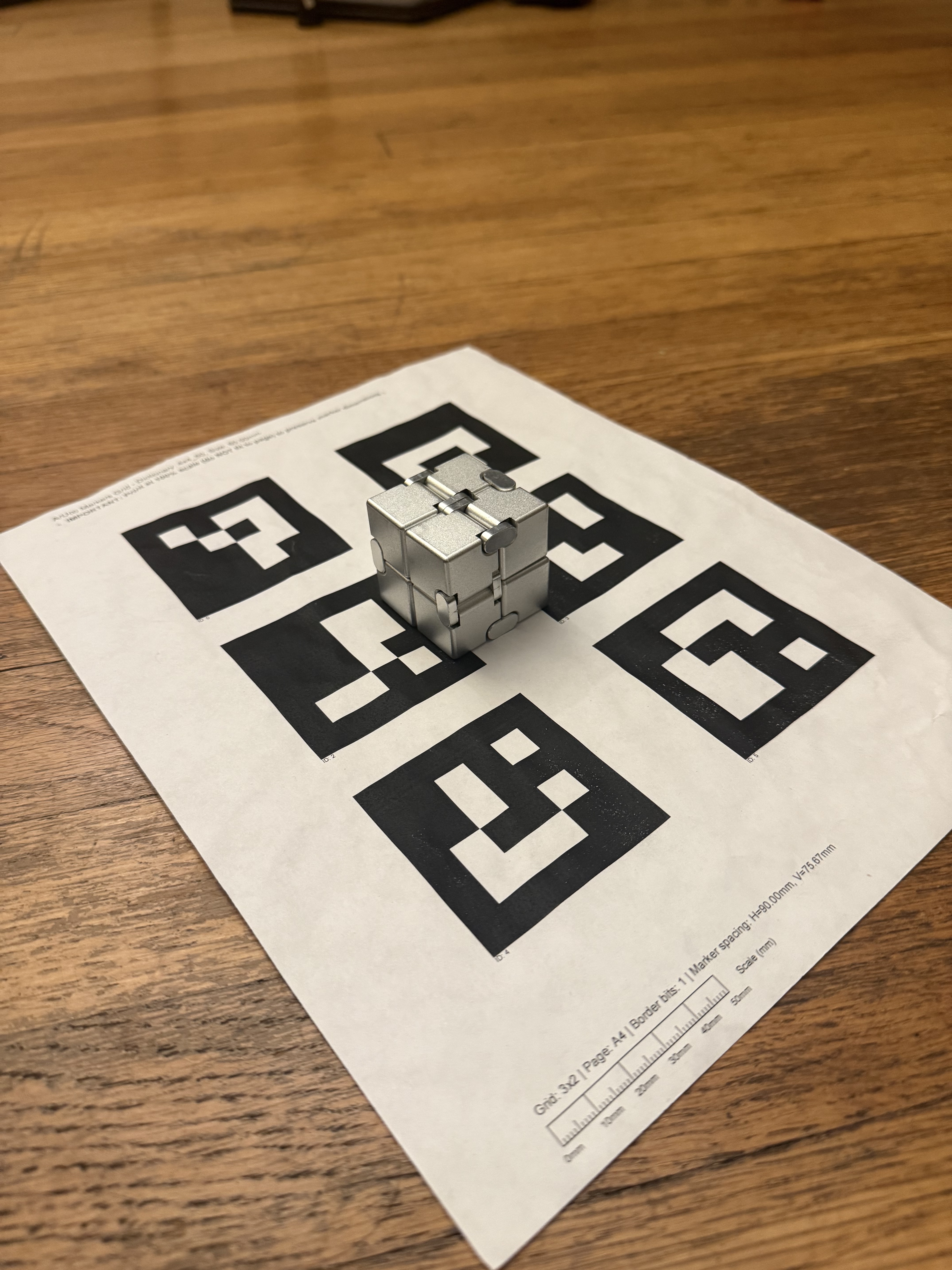
I printed the aruco tag sheet (since that's what the lububu set did) and placed my object next to it. I captured 30-50 images from different angles at a consistent distance (~10-20cm), ensuring uniform lighting and avoiding motion blur. However, these images were huge and hence were downsized later. Here's an example of the image I took.

0.3: Camera Pose Estimation

For each captured image, I detected the ArUco tag and used cv2.solvePnP() to estimate the camera's rotation (rvec) and translation (tvec) relative to the tag. I converted these to camera-to-world (c2w) transformation matrices by inverting the world-to-camera transform.

Deliverable: Viser visualization showing camera frustums positioned around the object with their captured images

0.4: Undistortion & Dataset Creation

I undistorted all images using cv2.undistort() to remove lens effects (pinhole camera assumption). To eliminate black borders, I used cv2.getOptimalNewCameraMatrix() with alpha=0 to crop to the valid pixel region and adjusted the principal point accordingly.

The final dataset was saved as my_data.npz with an 80/10/10 train/val/test split containing undistorted images, c2w matrices, and scaled focal length.

Part 1 — Fit a Neural Field to a 2D Image

Instead of storing an image as a grid of pixels, I trained a neural network to become the image itself. The network learns a continuous function that maps pixel coordinates (x, y) to RGB colors.

Model Architecture

Network Parameters:

Input: 2D coordinates (x, y) normalized to [0, 1]
Positional Encoding: L=10 (expands 2D → 42D using sinusoidal basis)
Hidden Layers: 4 fully connected layers, 256 neurons each, ReLU activation
Output: 3 RGB values with Sigmoid activation → [0, 1]
Learning Rate: 1e-2 (Adam optimizer)
Batch Size: 10,000 pixels per iteration
Total Iterations: 2000

Why Positional Encoding?

Standard MLPs struggle with high-frequency details. Sinusoidal Positional Encoding expands each coordinate into multiple frequency bands, allowing the network to learn both coarse structure and fine details.

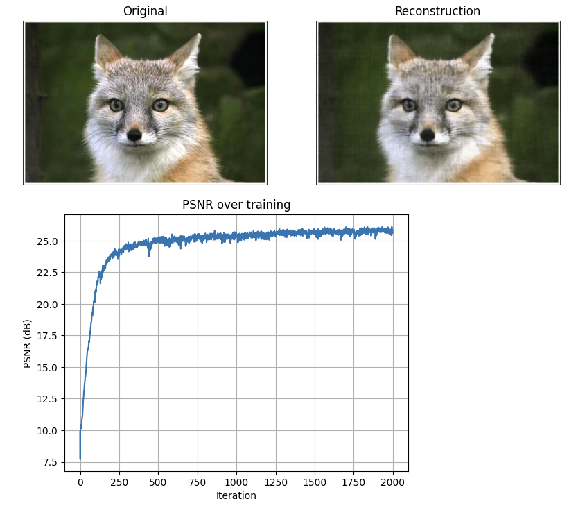
PE(x) = [x, sin(2⁰π·x), cos(2⁰π·x), ..., sin(2^(L-1)π·x), cos(2^(L-1)π·x)]

Results

Provided Test Image (Fox)

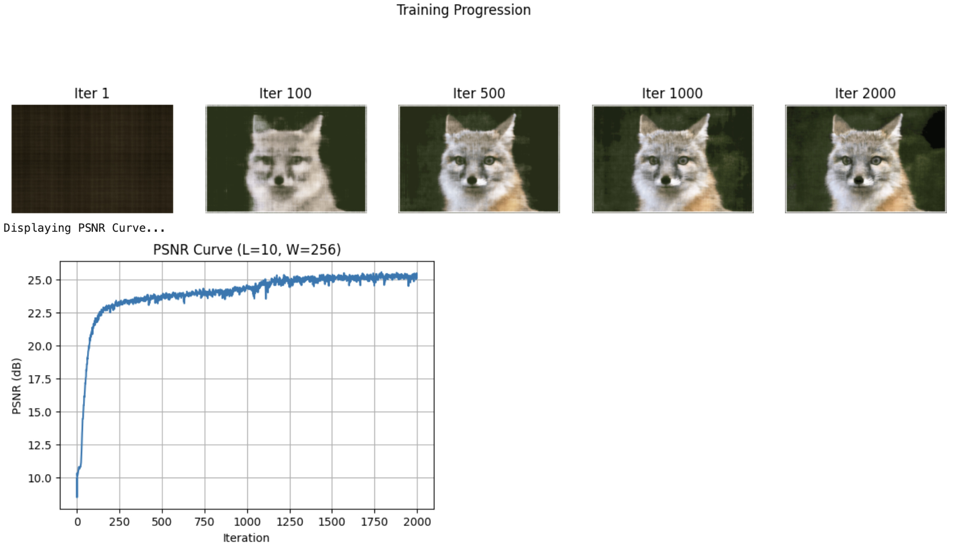
Fox Training Comparison — **Deliverable:** Left: Original, Right: Reconstruction, Bottom: PSNR

Fox Training Progression — **Deliverable:** Training progression showing convergence

Hyperparameter Sweep (Fox)

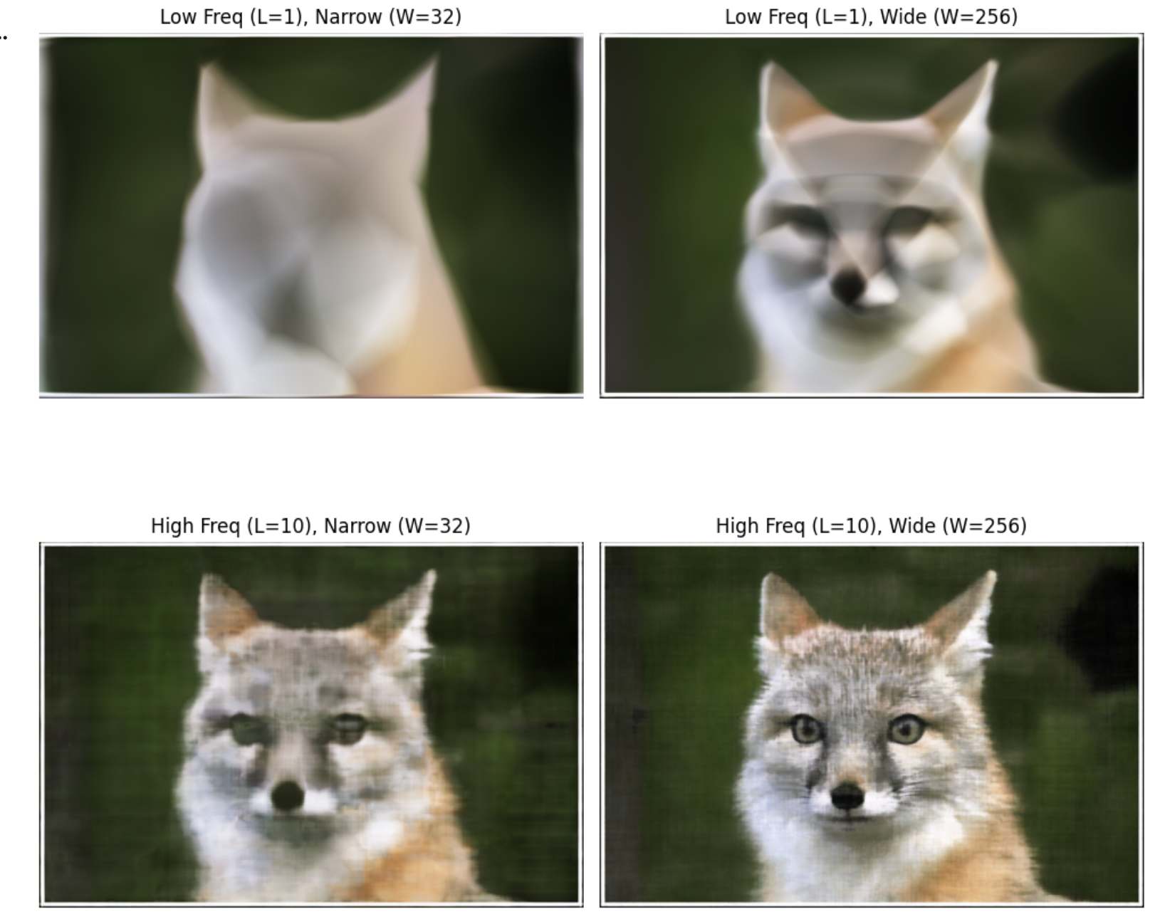
Deliverable: 2×2 grid showing effect of PE levels (L=1 vs L=10) and network width (W=32 vs W=256)

Custom Image (Elephant)

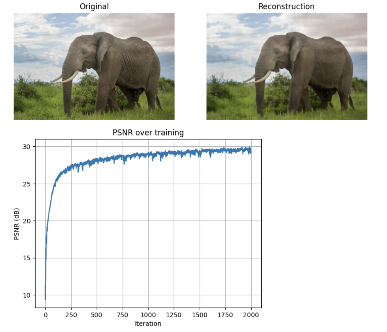
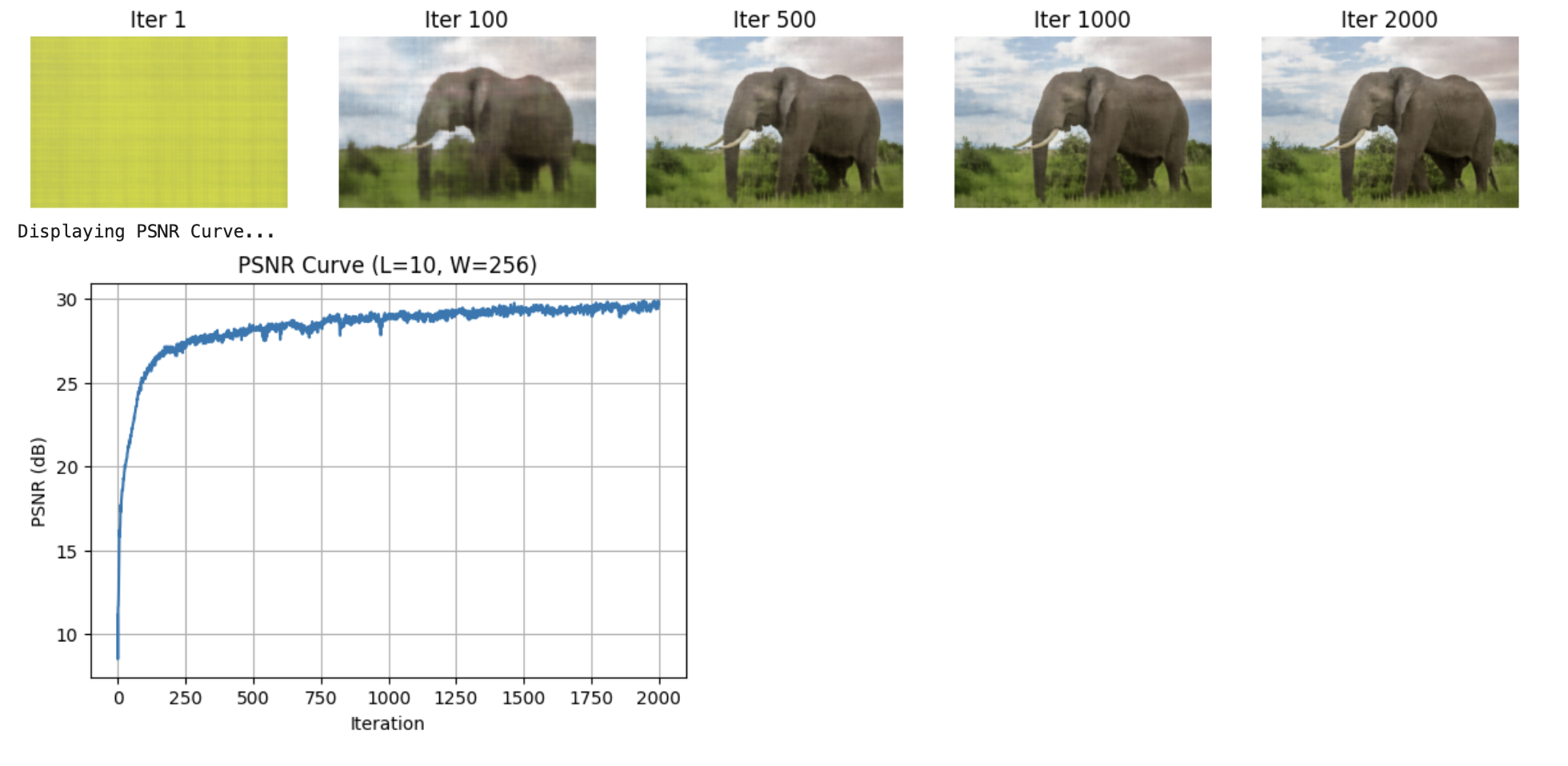
Elephant Training — **Deliverable:** Training on custom image

Elephant Progression — **Deliverable:** Iteration progression and PSNR curve

Hyperparameter Sweep (Elephant)

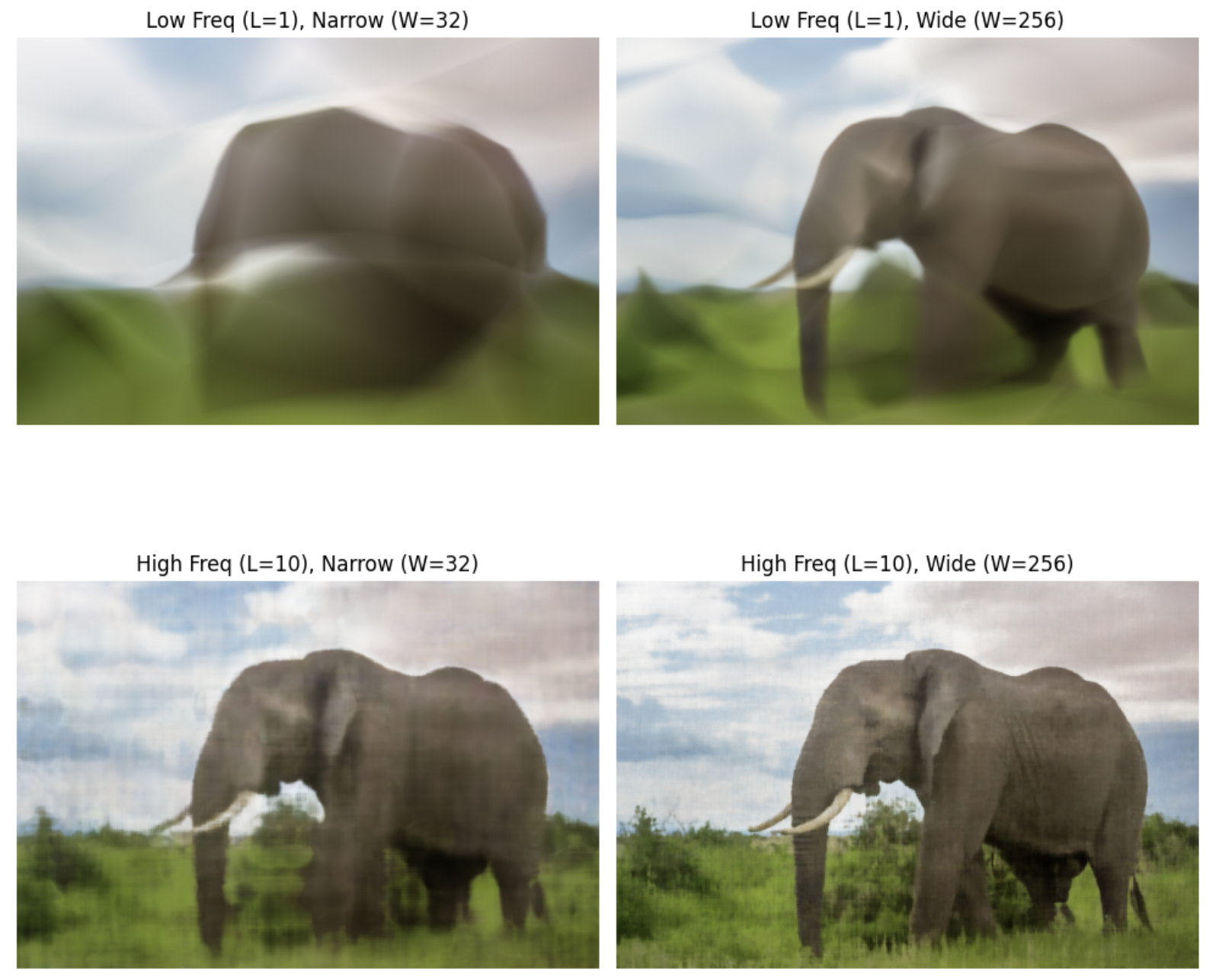
Deliverable: 2×2 grid showing hyperparameter effects on custom image

Key Observations:

Low L (frequency): Blurry results, misses fine details
High L: Sharp details, captures high-frequency content
Narrow width: Underfitting, poor reconstruction
Wide width: Better capacity, improved PSNR

Part 2 — Fit a Neural Radiance Field to a 3D Scene

Extending from 2D to 3D, the NeRF network now takes 5D input: 3D position (x, y, z) and 2D viewing direction. It outputs volume density (σ) and view-dependent RGB color.

2.1: Create Rays from Cameras

I implemented three core functions to convert pixels to rays:

pixel_to_camera(K, uv, s): Unprojects pixel coordinates to camera space using intrinsic matrix K
transform(c2w, x_c): Transforms points from camera space to world space using c2w matrix
pixel_to_ray(K, c2w, uv): Generates ray origin and normalized direction for each pixel

Key Implementation Detail: Ray origin is extracted from c2w translation component: o = c2w[:3, 3]. Ray direction is computed by transforming a camera-space point at depth s=1 to world space, then normalizing: d = (x_w - o) / ||x_w - o||

2.2: Stratified Sampling Along Rays

To avoid aliasing and ensure continuous coverage, I implemented stratified sampling with random jitter:

Divide depth range [near, far] into N equal bins
Compute bin boundaries as midpoints between samples
Randomly perturb sample positions within each bin (training only)
Compute 3D points: pts = rays_o + rays_d × z_vals

For Lego dataset: NEAR=2.0, FAR=6.0, N_SAMPLES=128

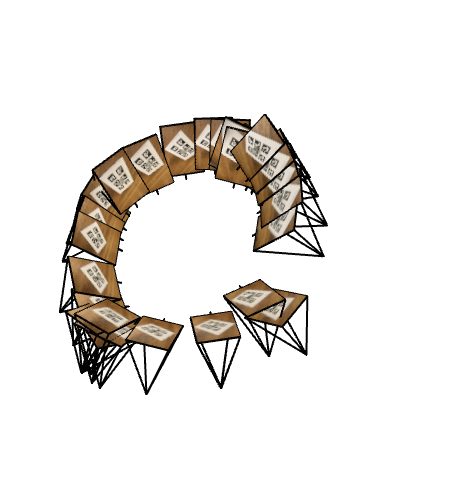
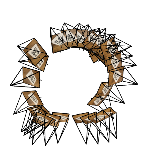
2.3: Visualization of Rays and Samples

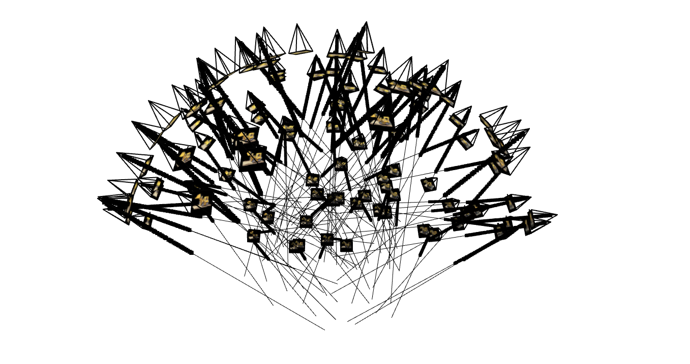
Viser Ray Sampling — **Deliverable:** Viser visualization showing camera frustums (black), 100 sampled rays (white lines), and stratified sample points (green dots) for the Lego dataset

Verification Checklist:

✅ All camera frustums positioned correctly around object
✅ Rays originate from camera centers and point into scene
✅ Sample points evenly distributed along rays from near to far
✅ Ray directions properly normalized

2.4: NeRF Network Architecture

Network Parameters:

Depth (D): 8 hidden layers
Width (W): 256 neurons per layer
Position Encoding: L_pos=10 (3D → 63D)
Direction Encoding: L_dir=4 (3D → 27D)
Skip Connection: At layer 5 (concatenate input back)
Output: Density (σ with ReLU) + View-dependent RGB (Sigmoid)

Architecture Flow:

Input (x,y,z) → PE(63D) → Layers 0-4 → [Skip: concat with PE] → Layers 5-7 → Branch 1: Density Head (σ) → Branch 2: Feature → [concat with dir PE] → Color Head (RGB)

2.5: Volume Rendering Equation

The core volume rendering equation aggregates density and color samples along each ray:

C(r) = Σ[i=1 to N] T_i · α_i · c_i where: α_i = 1 - exp(-σ_i · Δt) [opacity at sample i] T_i = Π[j<i] (1 - α_j) [transmittance: light reaching sample i] Δt = distance between samples

Implementation Steps:

Compute alpha: Convert density to opacity over step size
Compute transmittance: Cumulative product of (1-alpha), shifted right with T_0=1
Compute weights: w_i = T_i × α_i
Accumulate color: Final RGB = Σ(weights × colors)

Validation: ✅ Passed numerical test with random batches (rtol=1e-4, atol=1e-4)

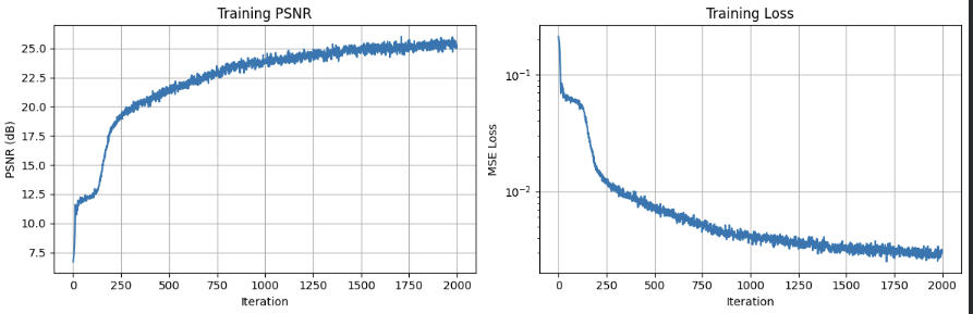
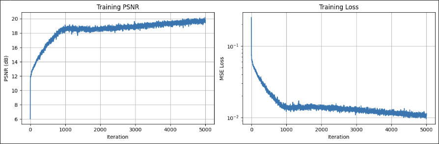
2.6: Training on Lego Bulldozer Dataset

Training Hyperparameters:

Dataset: 100 training images, 200×200 resolution
Batch Size: 4096 rays per iteration
Learning Rate: 5e-4 (Adam) with MultiStep scheduler
Iterations: 2000-5000
Near/Far: 2.0 to 6.0
Samples per Ray: 128

Training Progression

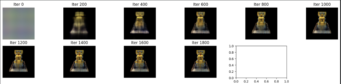
Deliverable: Predicted views showing progressive reconstruction quality

Lego PSNR — **Deliverable:** PSNR curve on validation set (achieved 23+ dB)

Lego Spiral — **Deliverable:** Novel view synthesis using test camera poses

Training With Custom Data

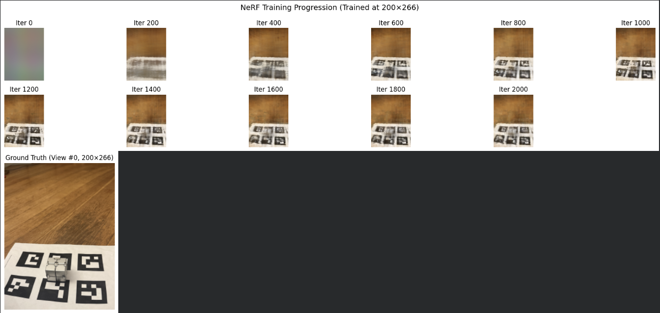
Deliverable: Predicted custom views showing progressive reconstruction quality

Custom PSNR — **Deliverable:** PSNR curve on validation set (achieved almost 20+ dB)

Key Takeaways:

I probably shouldn't have used a shiny object! I think that definitely messed stuff up
Camera calibration accuracy directly impacts reconstruction quality
Scene-specific near/far planes are critical for efficient depth sampling
View-dependent effects (specular highlights) require proper direction encoding
Longer training and higher sample counts improve fine geometric details
Focal length must be scaled proportionally when resizing images

Challenges & Lessons Learned

Challenge 1: Coordinate System Confusion

The provided spiral generation code assumed standard Y-up coordinates, but my cameras were positioned in negative-Y space. I fixed this by implementing a robust look_at_origin() function that computes correct rotation matrices regardless of camera position, ensuring cameras always point at the origin.

Challenge 2: Focal Length Scaling

When training on resized images, I initially forgot to scale the focal length, causing a "zoom lens" effect where renders only showed a tiny patch. Fix: focal_render = focal_train × (W_render / W_train)

Challenge 3: DON'T USE SHINY OBJECTS

Self explanatory — the shiny surface caused inconsistent color observations from different angles, making it hard for the network to learn a coherent representation. Next time, I'll pick a matte object!