CS180 Class Repository — Garv Goswami

Overview

The goal of this assignment was to implement homography estimation, inverse warping with nearest neighbor and bilinear interpolation, rectification, and finally blend multiple photos into mosaics using feathered alpha masks. I avoided the disallowed high-level warping APIs (e.g., cv2.findHomography, cv2.warpPerspective, skimage.transform.warp) and wrote the core pieces from scratch.

A.1 — Shoot the Pictures

I shot a bunch overlapping sequences by rotating the camera about (roughly) a fixed center of projection to induce projective transforms. The reason I took so many was to be able to compile the best results for when it's time to generate mosaics. Below are four sets (more than the required two):

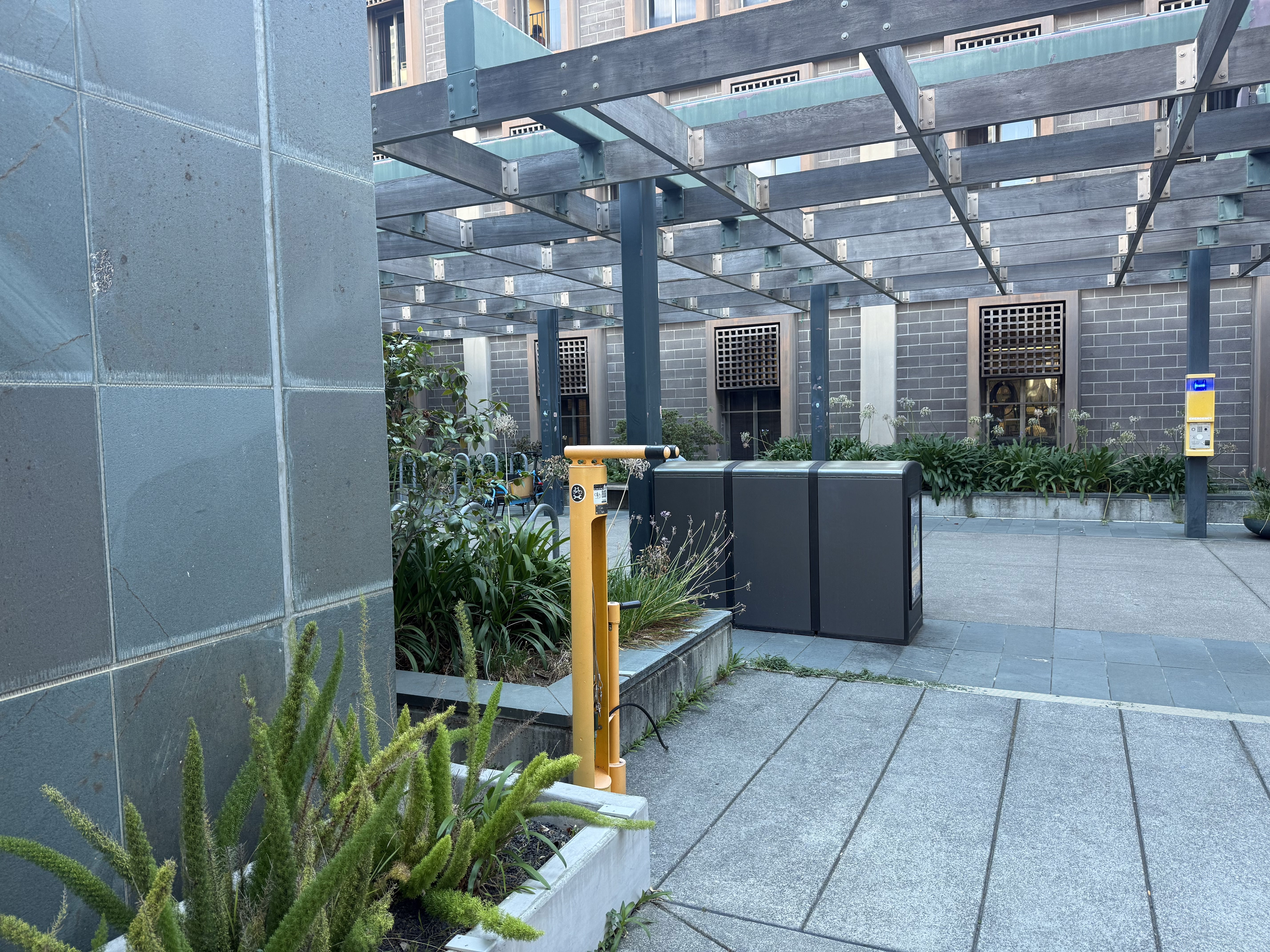
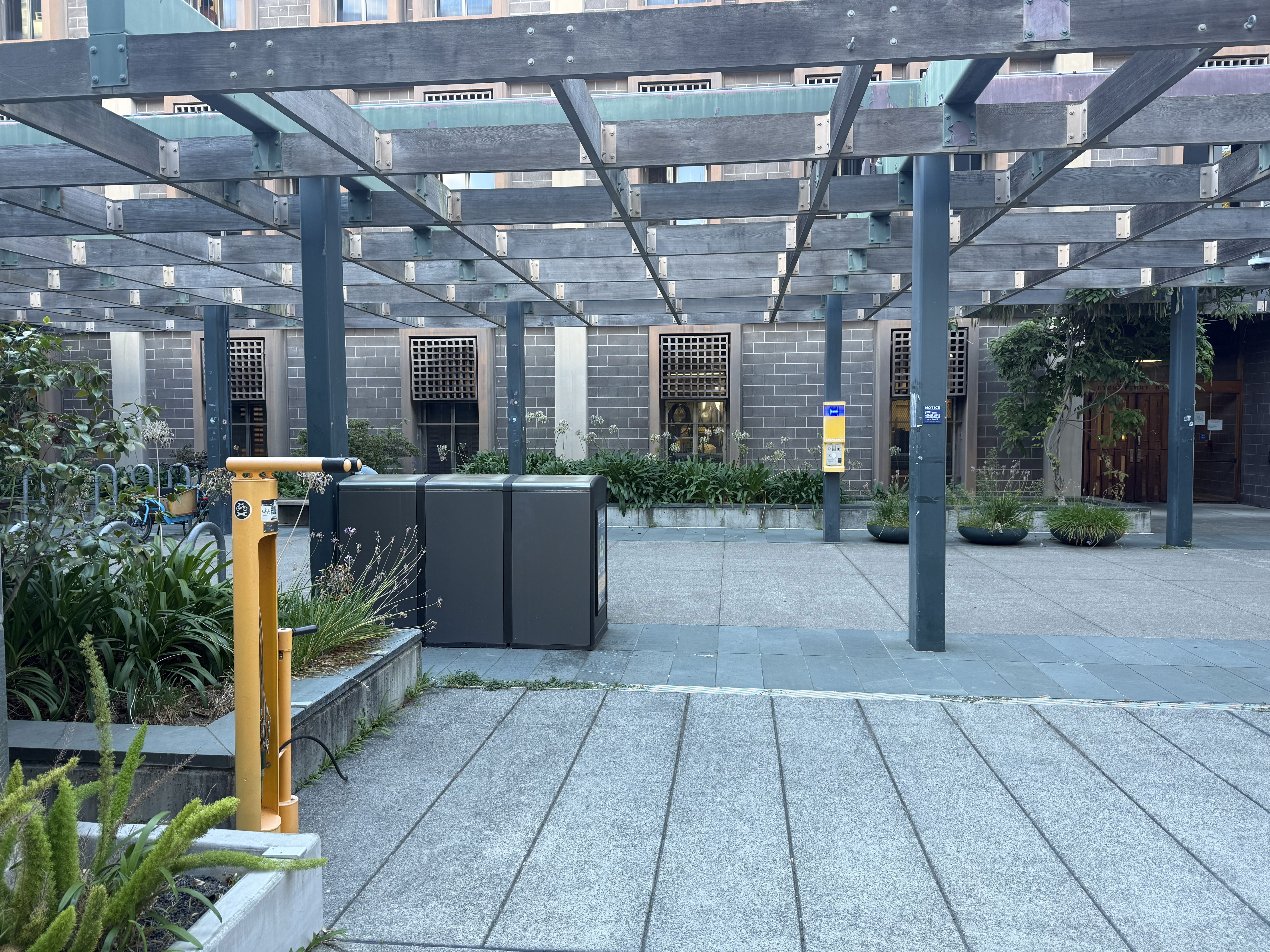
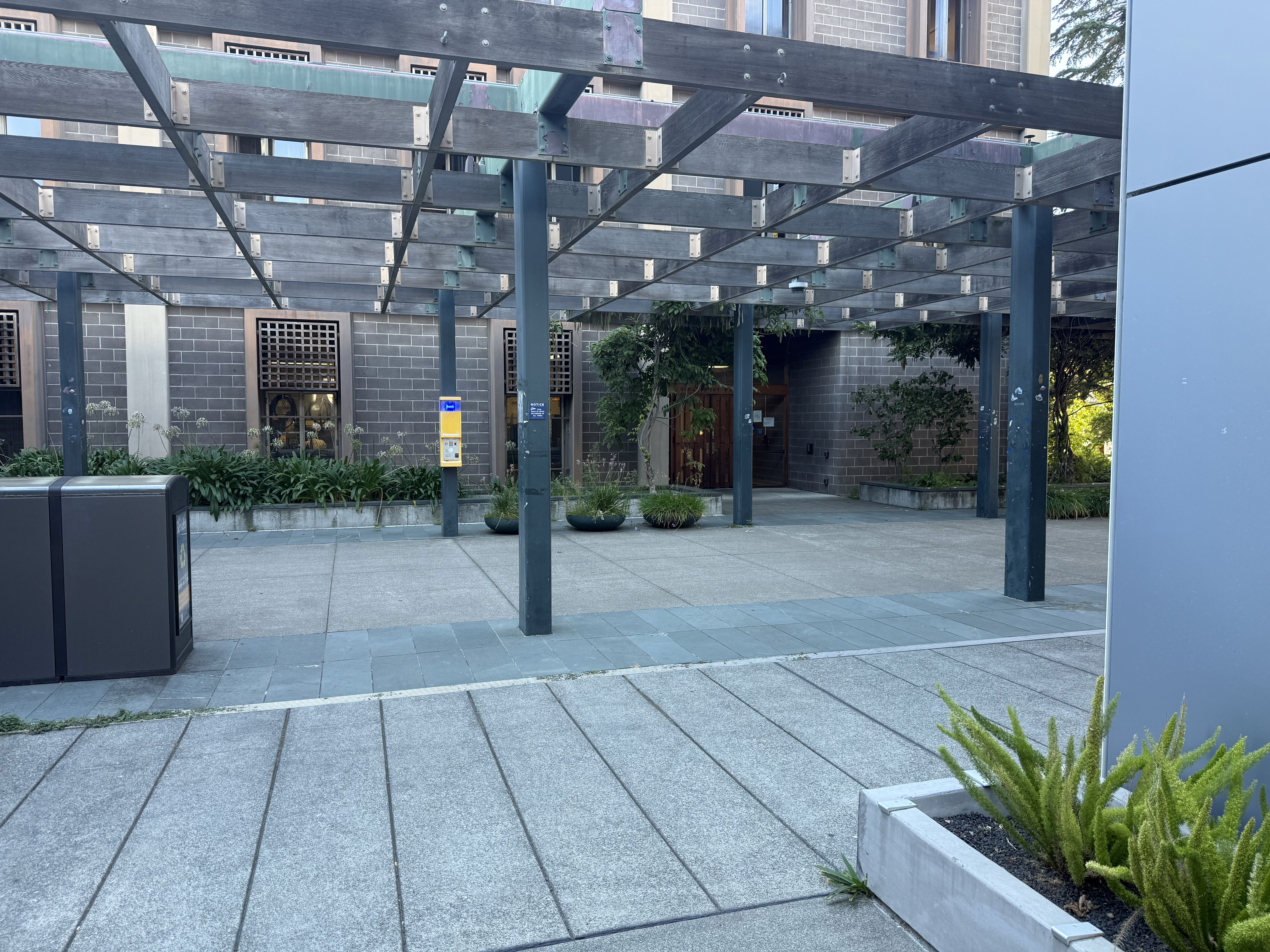
Set 1 — Breezeway

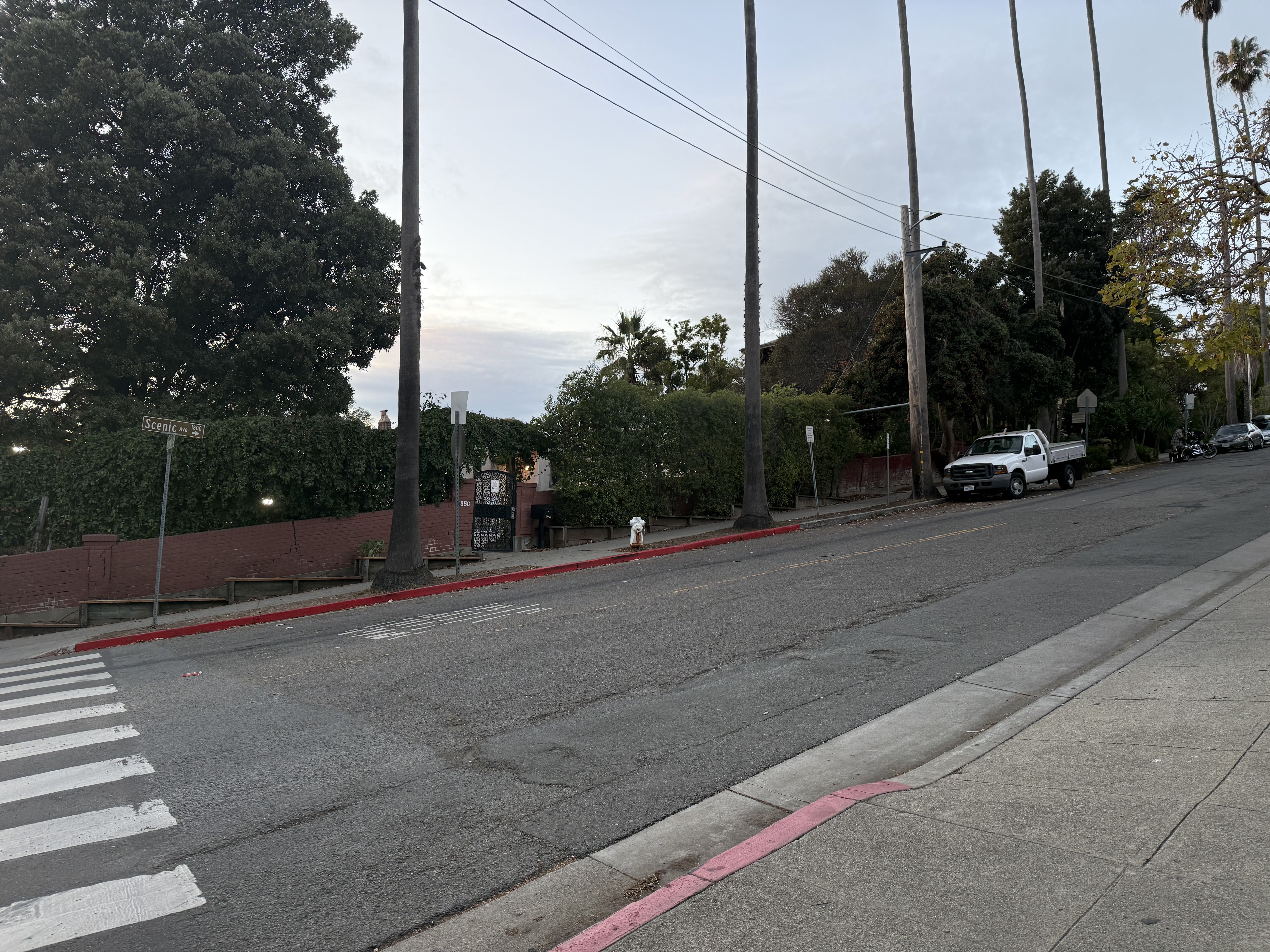
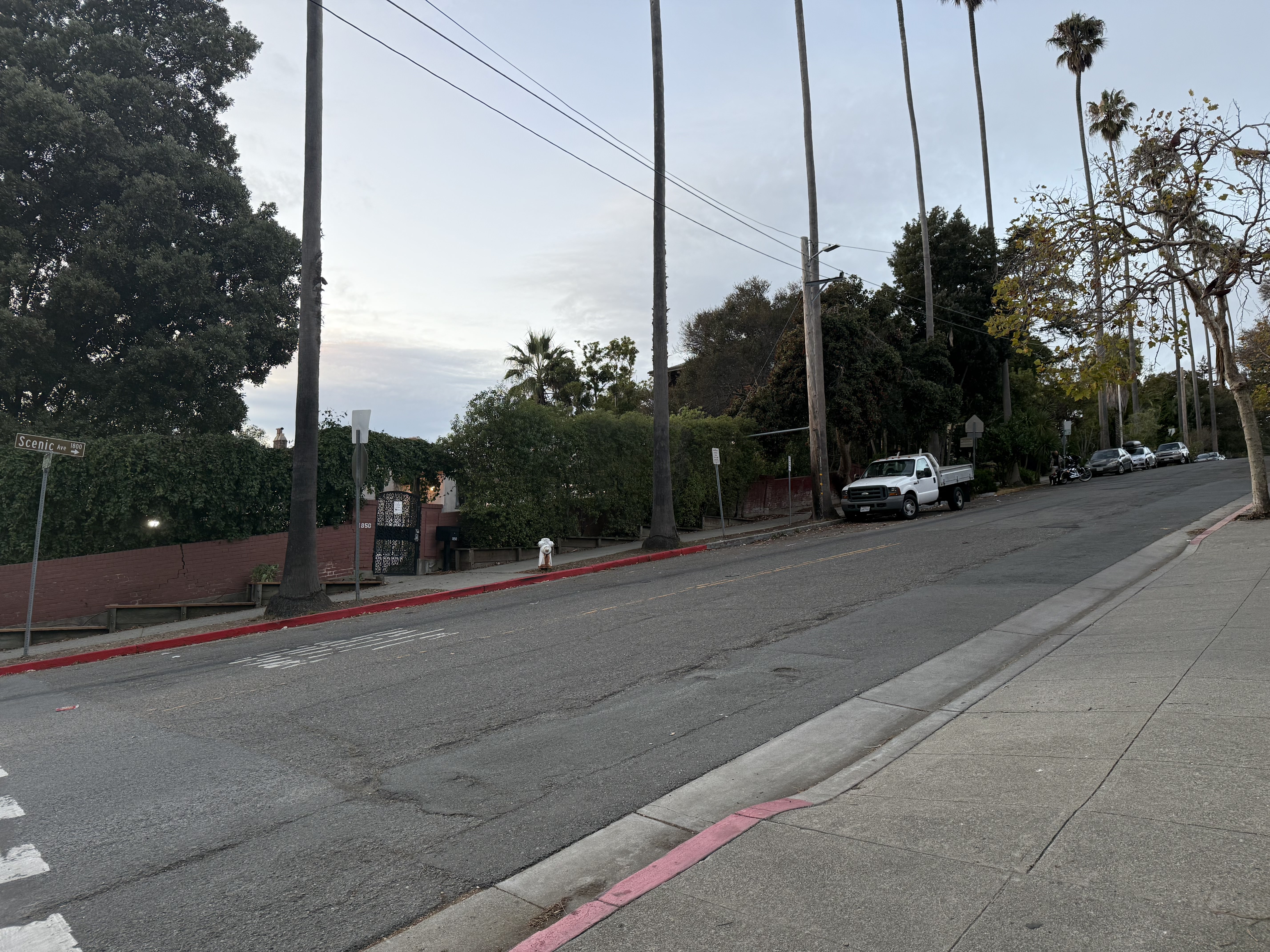
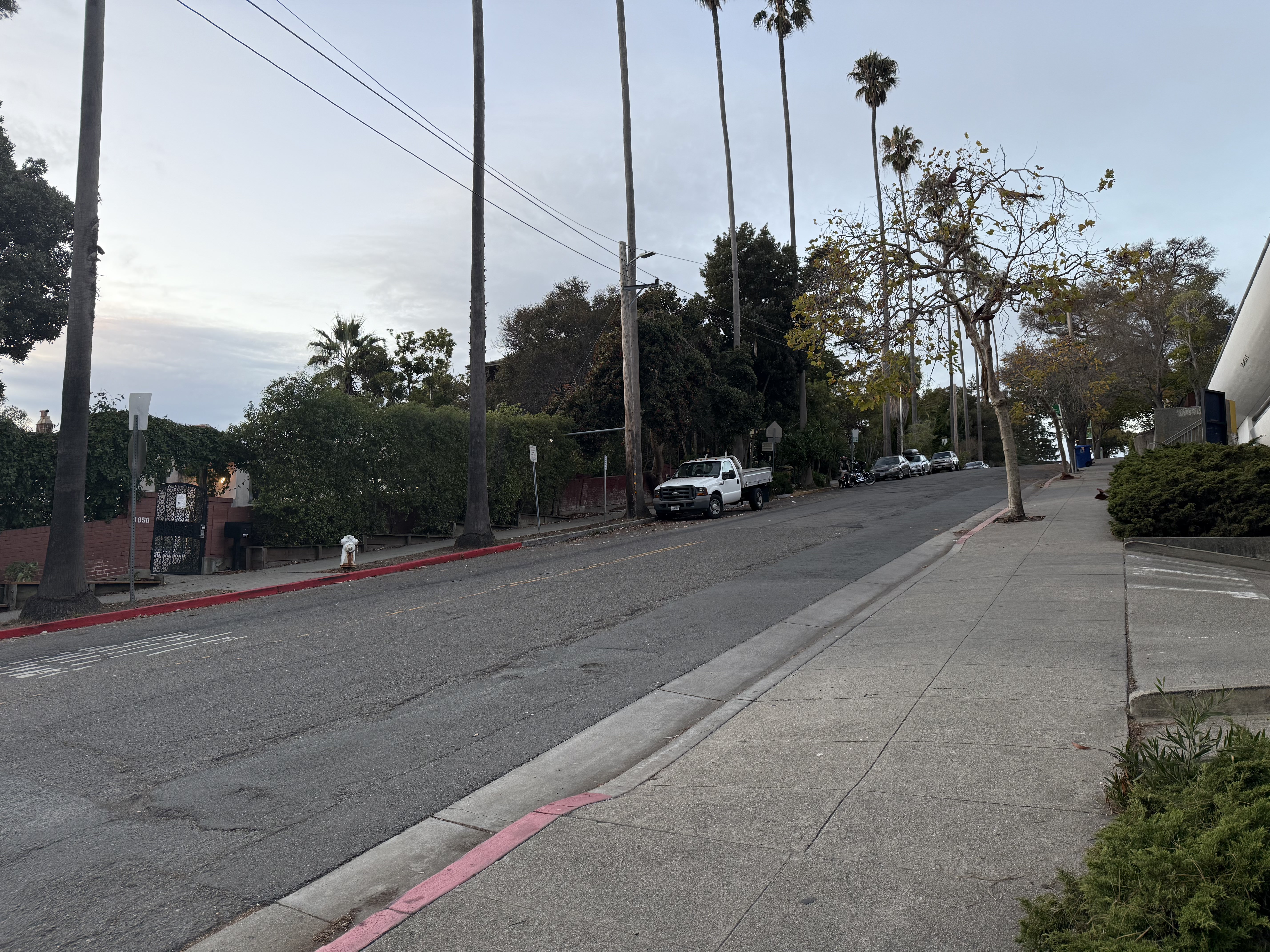
Set 2 — Scenic

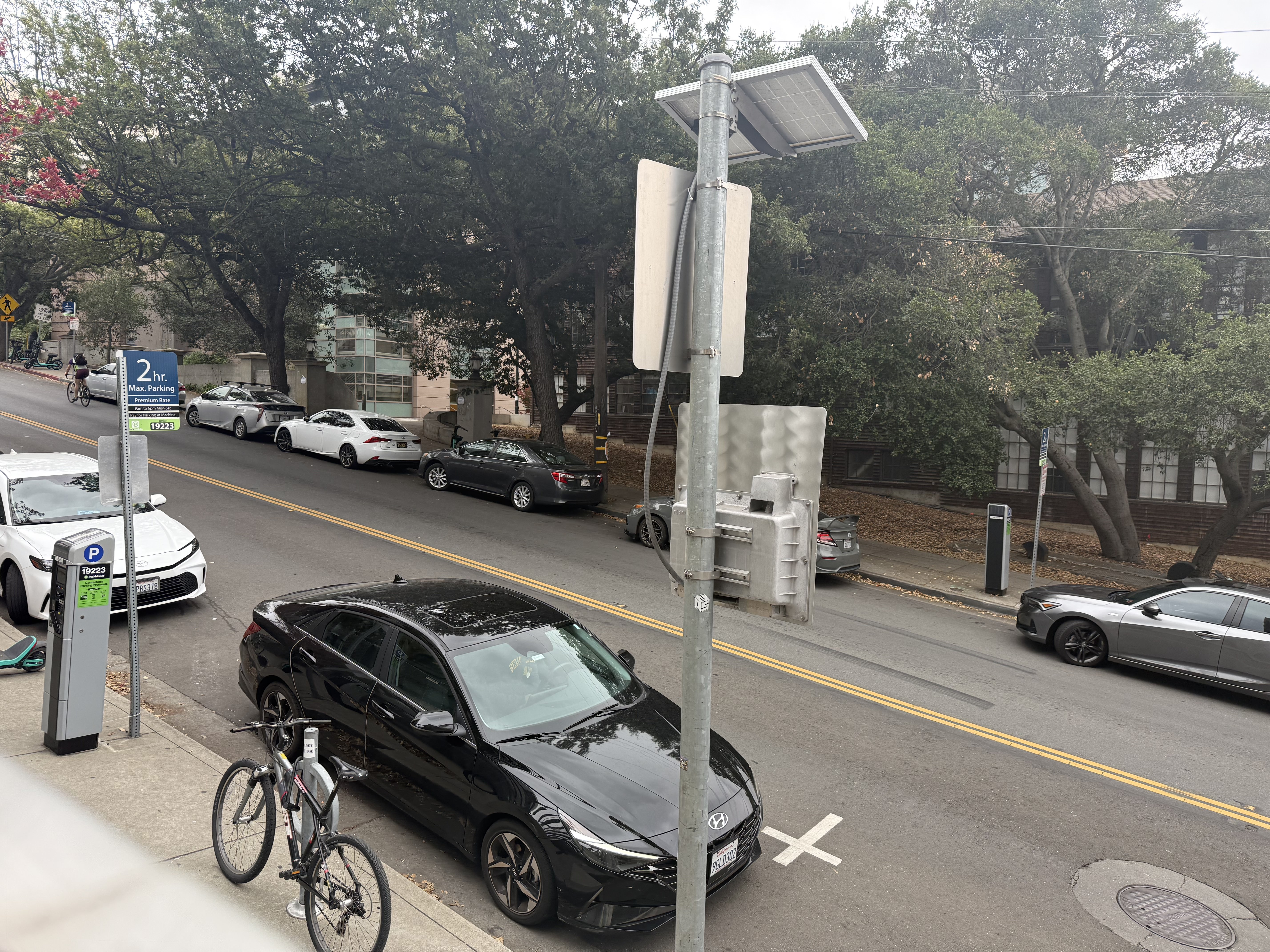
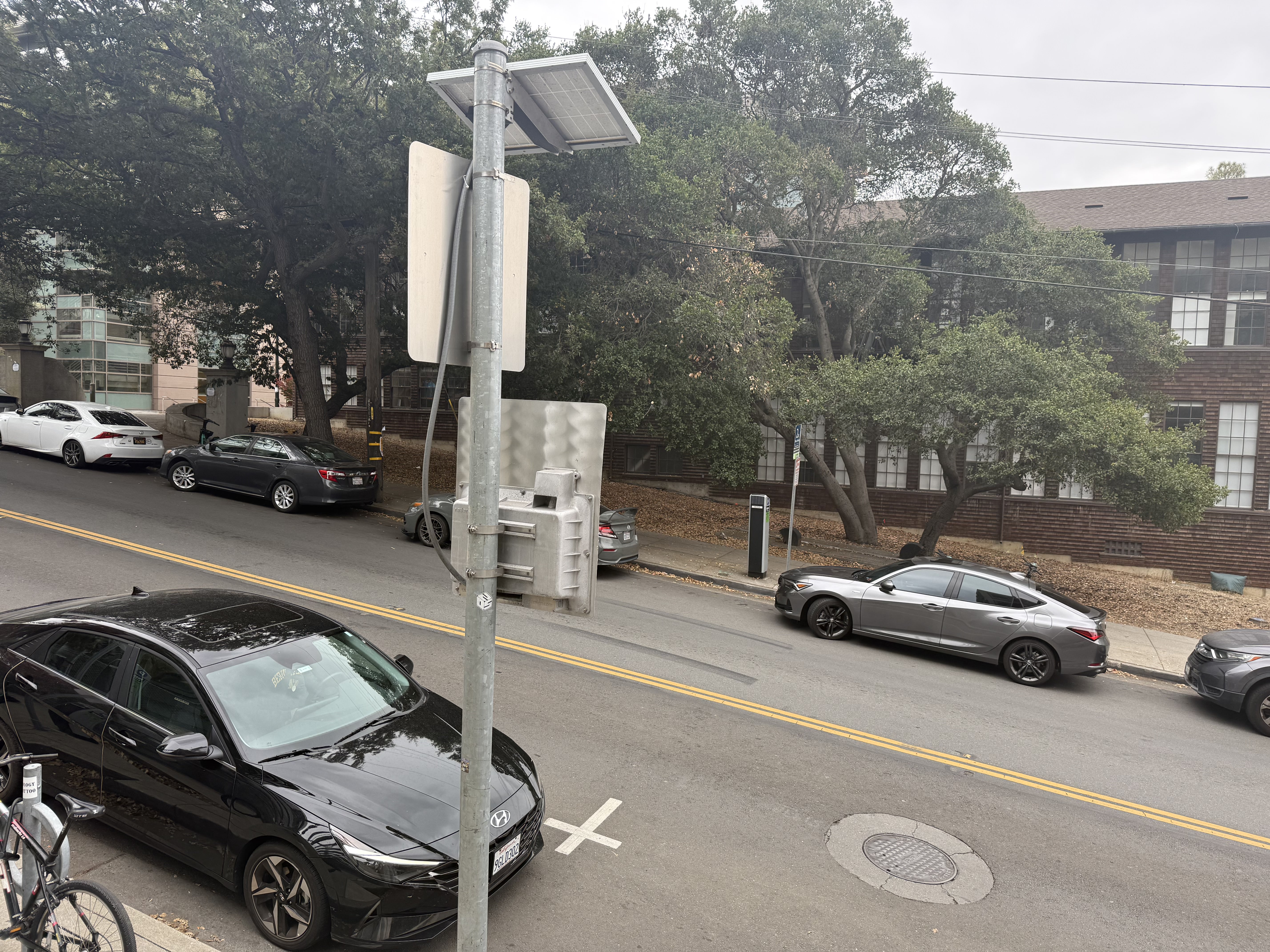
Set 3 — Hearst

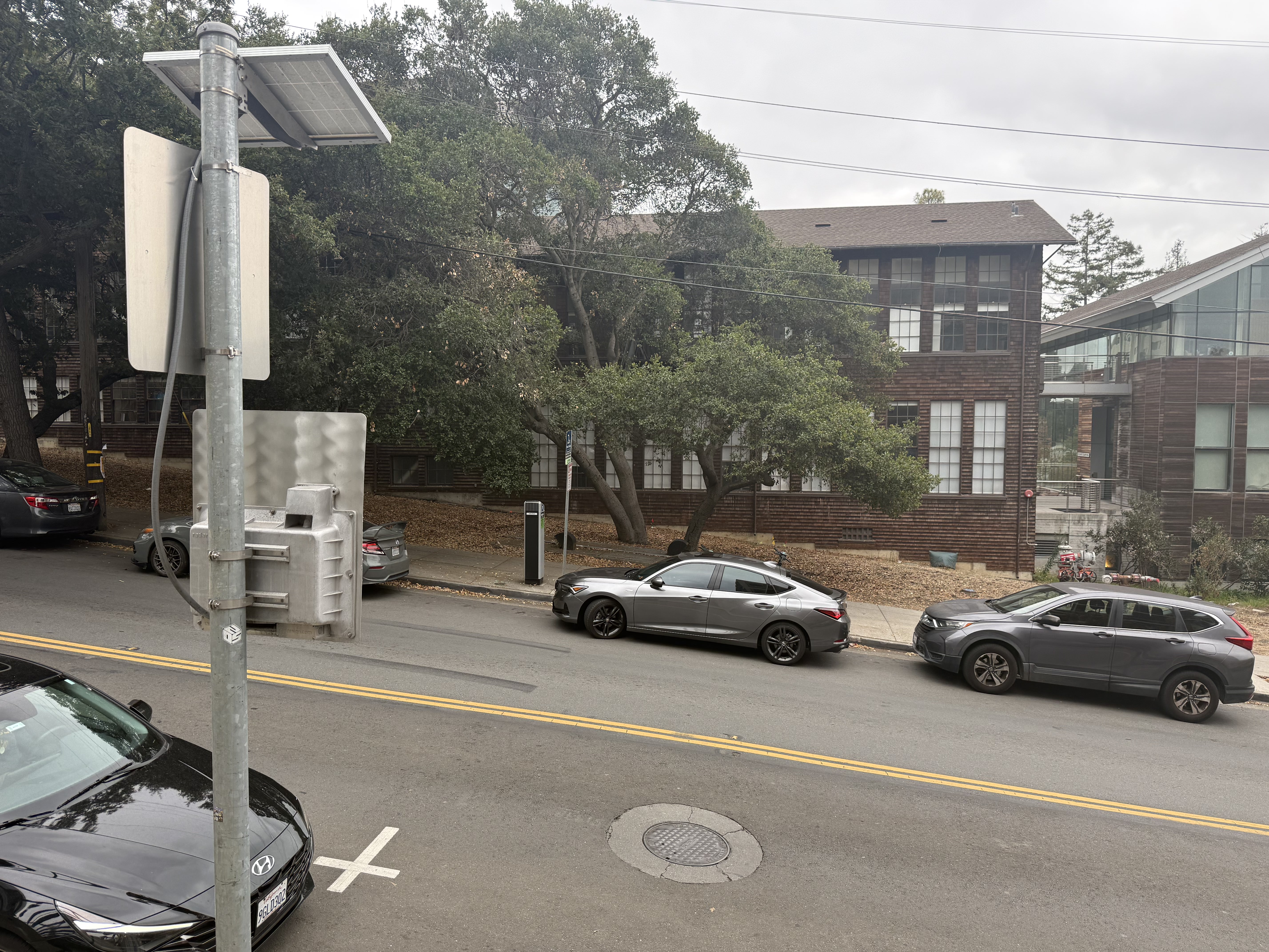
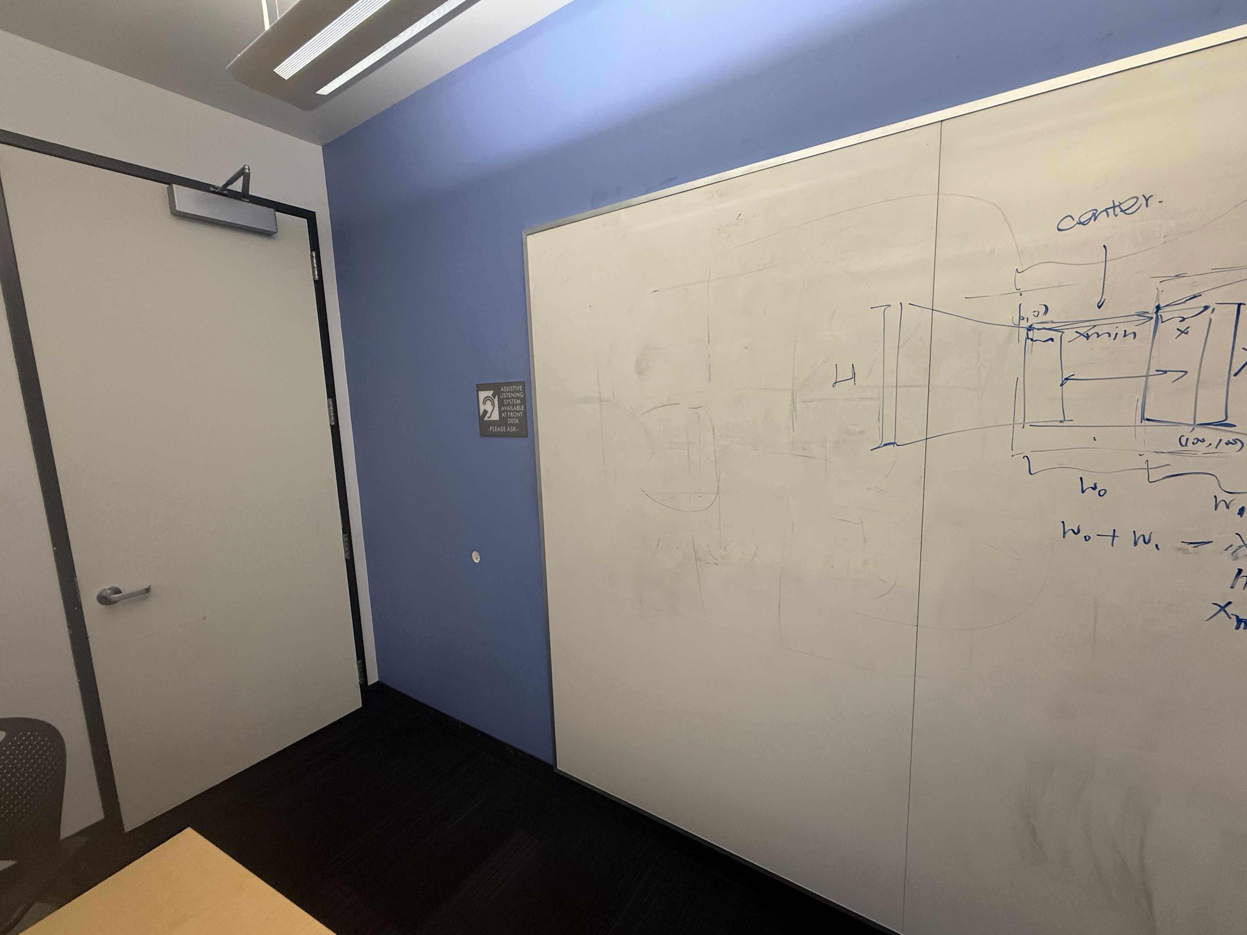
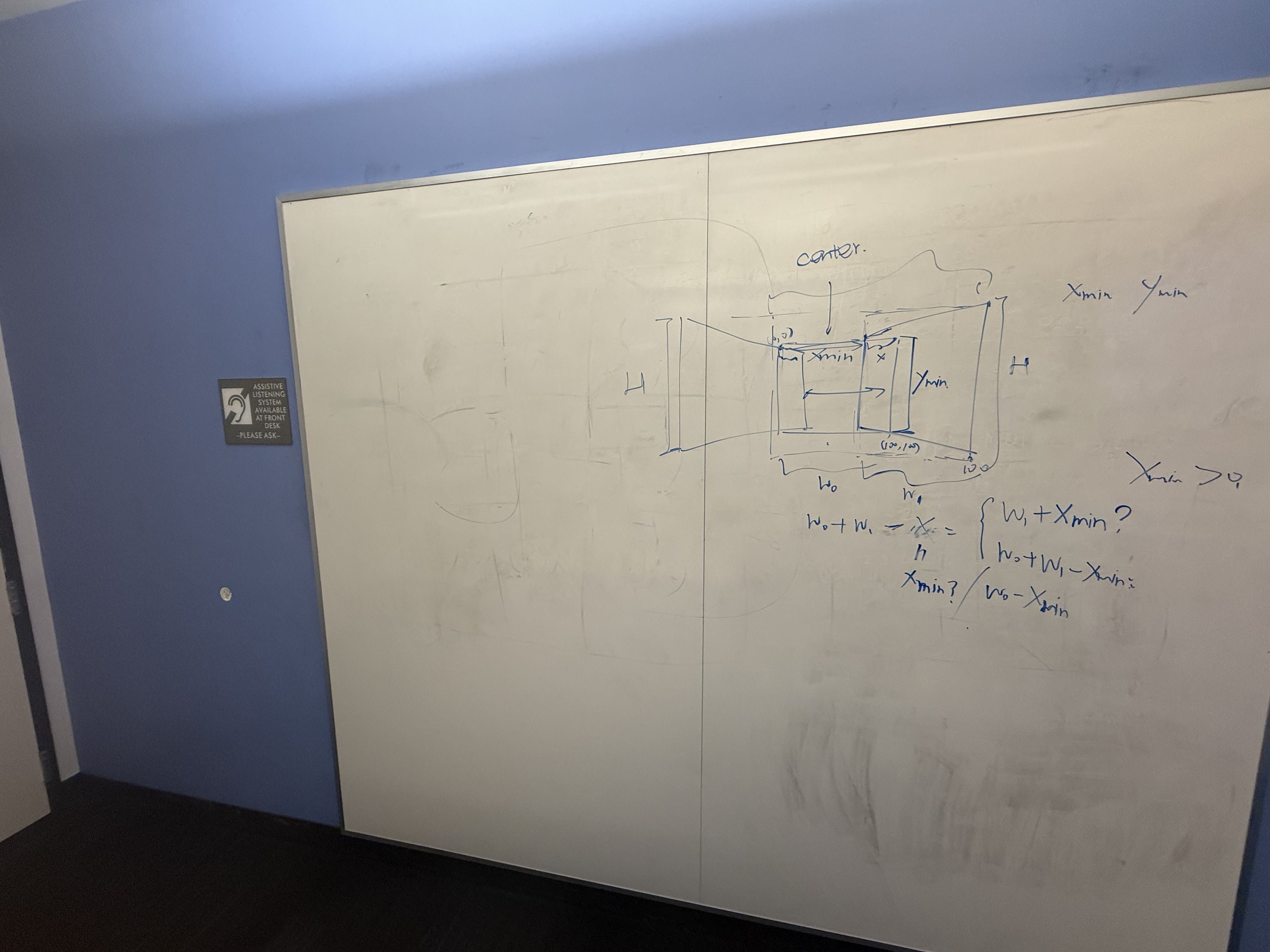
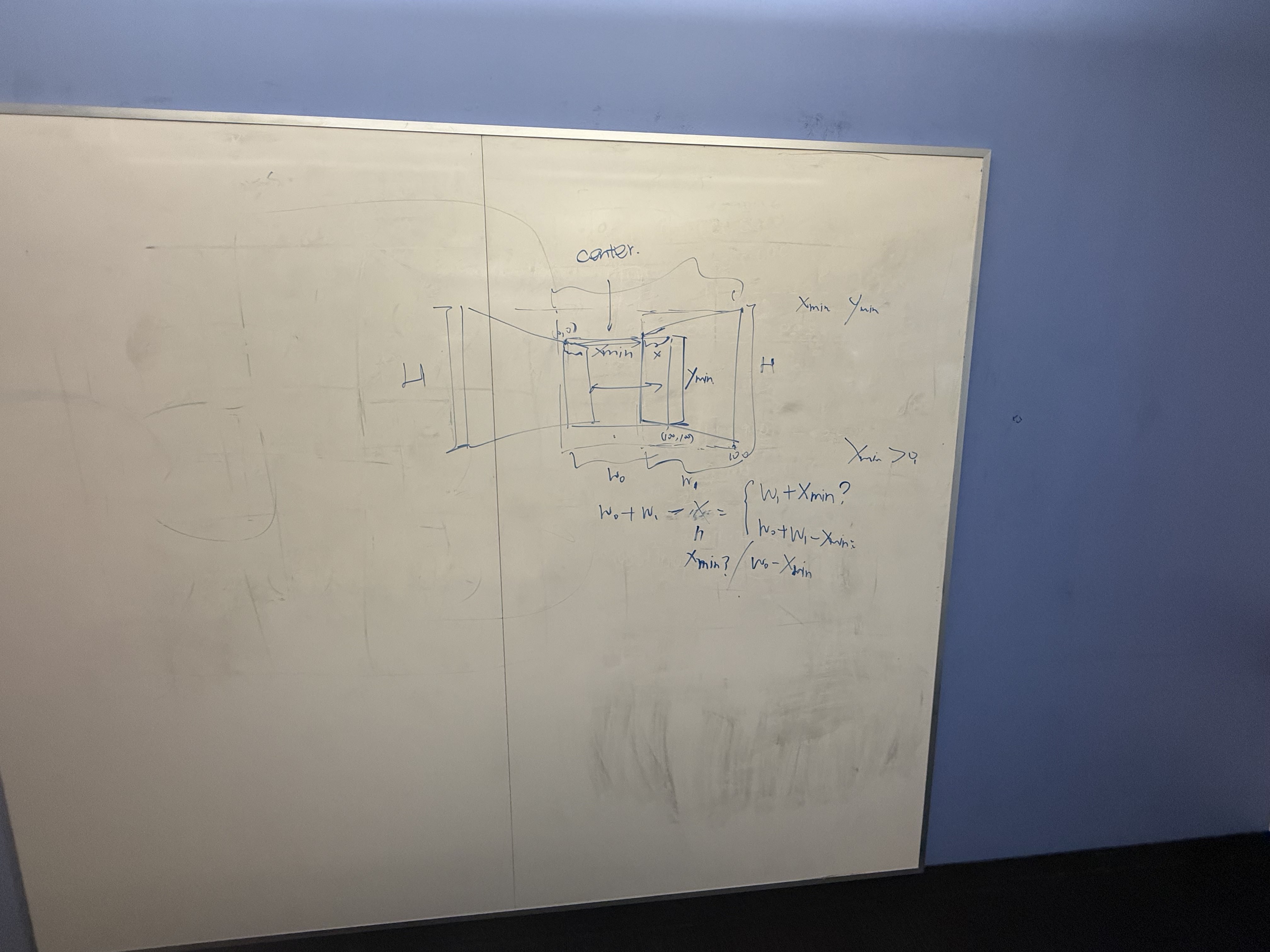
Set 4 — Whiteboard / Indoor

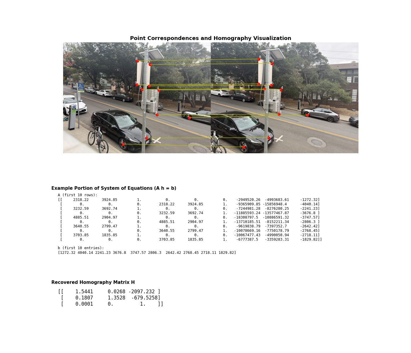
A.2 — Recover Homographies

I solve for the 3×3 homography H using a least-squares nullspace solution to A h = 0 from ≥4 correspondences (collected with matplotlib.ginput). I also visualize correspondences, show an excerpt of the linear system, and print the recovered H. Here’s the deliverable figure:

Core routine (trimmed to the essentials):

def computeH(im1_pts, im2_pts):
        # * num_points is just the number of points that we select, the more the better I'm pretty sure?
    
        #! Remember that the overall goal here is for two points in different images, we can use the homography matrix H to map the same pixel in the first photo to one in the second phone
        # TODO: Confirm the above in OH 
    
    
        #TODO: 10/10 Just talked to my friend and apparently I was allowed to use a built-in least-squares here. Unfortunate.
        num_points = im1_pts.shape[0]
        A = []
    
        for i in range(num_points):
    
        #* Each point pair giives us two equations from the projection relations
            x, y = im1_pts[i, 0], im1_pts[i, 1]
            x_2, y_2 = im2_pts[i, 0], im2_pts[i, 1]
            
            A.append([x, y, 1, 0, 0, 0, -x*x_2, -y*x_2, -x_2])
    
            A.append([0, 0, 0, x, y, 1, -x*y_2, -y*y_2, -y_2])
        
        #* A should have shape (2 x N, 9) after all that and we can conver to a numpy array
        A = np.array(A)
    
        #* Now we solve Ah = 0 using the svd bc we want a vec that lies in the null space of A
        #* SVD factorizes A = USV^T and the least squares minimizer is the right singular vec of the smallest singular val of A
        U, S, Vt = np.linalg.svd(A)
        #* Then we just fix the scale and reshape
        h = Vt[-1, :]
        h = h / h[-1] 
    
        H = h.reshape(3, 3)
    
        return H
    

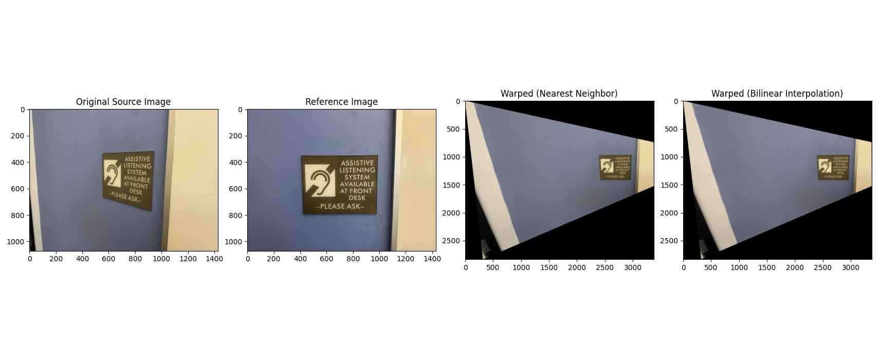
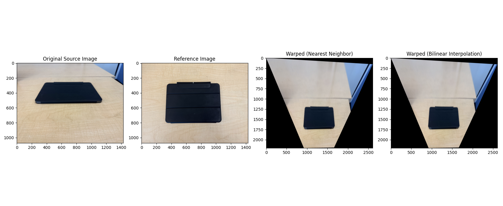
A.3 — Warp the Images + Rectification

I implemented inverse warping with both interpolation methods: nearest neighbor (fast but blocky) and bilinear (slower but smoother). To avoid holes, I invert the mapping from output pixels back to source coordinates and sample there. To be clear, the point of these interpolations is because warping lands us at non-integer pixel locations, and for each output pixel we need to map back to the source, which is where interpolation matters. Nearest Neighbor is exactly what it sounds like and uses the value of the single closest pixel input. Bilinear averages teh 4 neigbors with weights based on distance and takes longer, but gives a smoother result.

• warpImageNearestNeighbor(img, H)
• warpImageBilinear(img, H)

As a sanity check, I performed rectification on two images (making a planar object frontal-parallel).

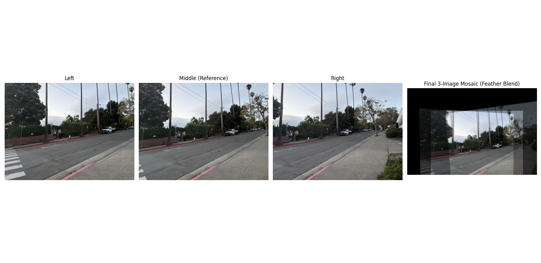
A.4 — Blend Images into Mosaics

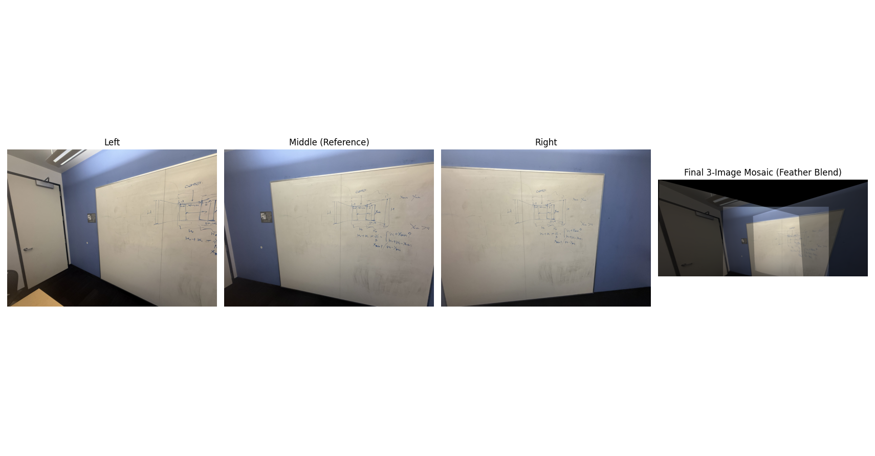
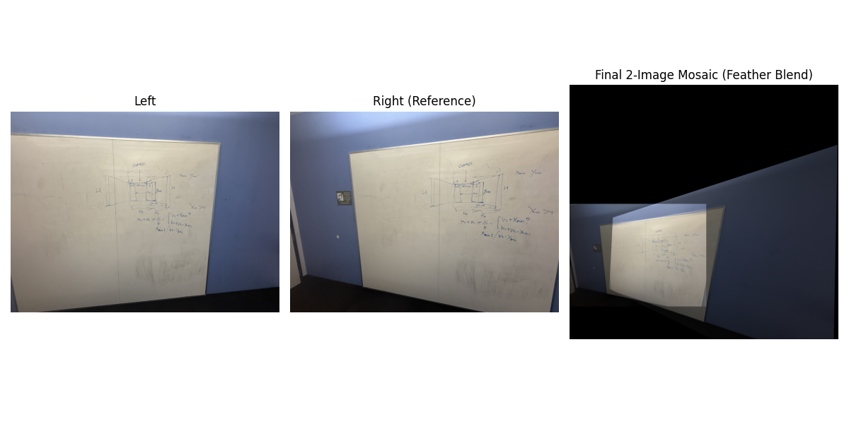
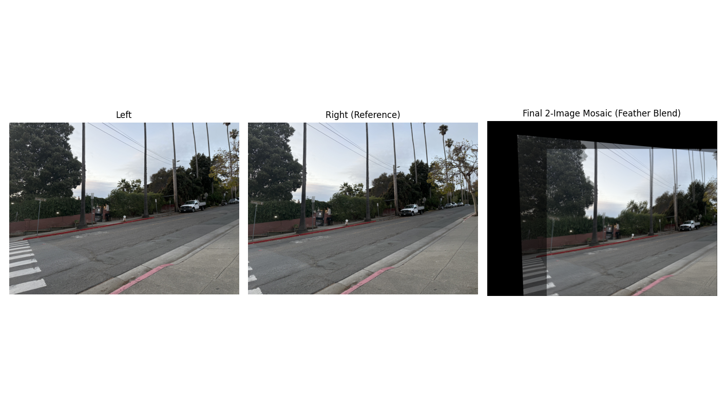
After warping into a common canvas (using the predicted global bounding box and a translation offset), I blend with simple feathering: set an alpha mask that falls off from image center to borders, and compute a per-pixel weighted average. Below are three mosaics with their source images.

Mosaic 1 — Scenic (3 images)

Mosaic 2 — Whiteboard (3 images)

Mosaic 2.1 — Whiteboard (2 images)

Mosaic 3 — Breezeway (2 images)

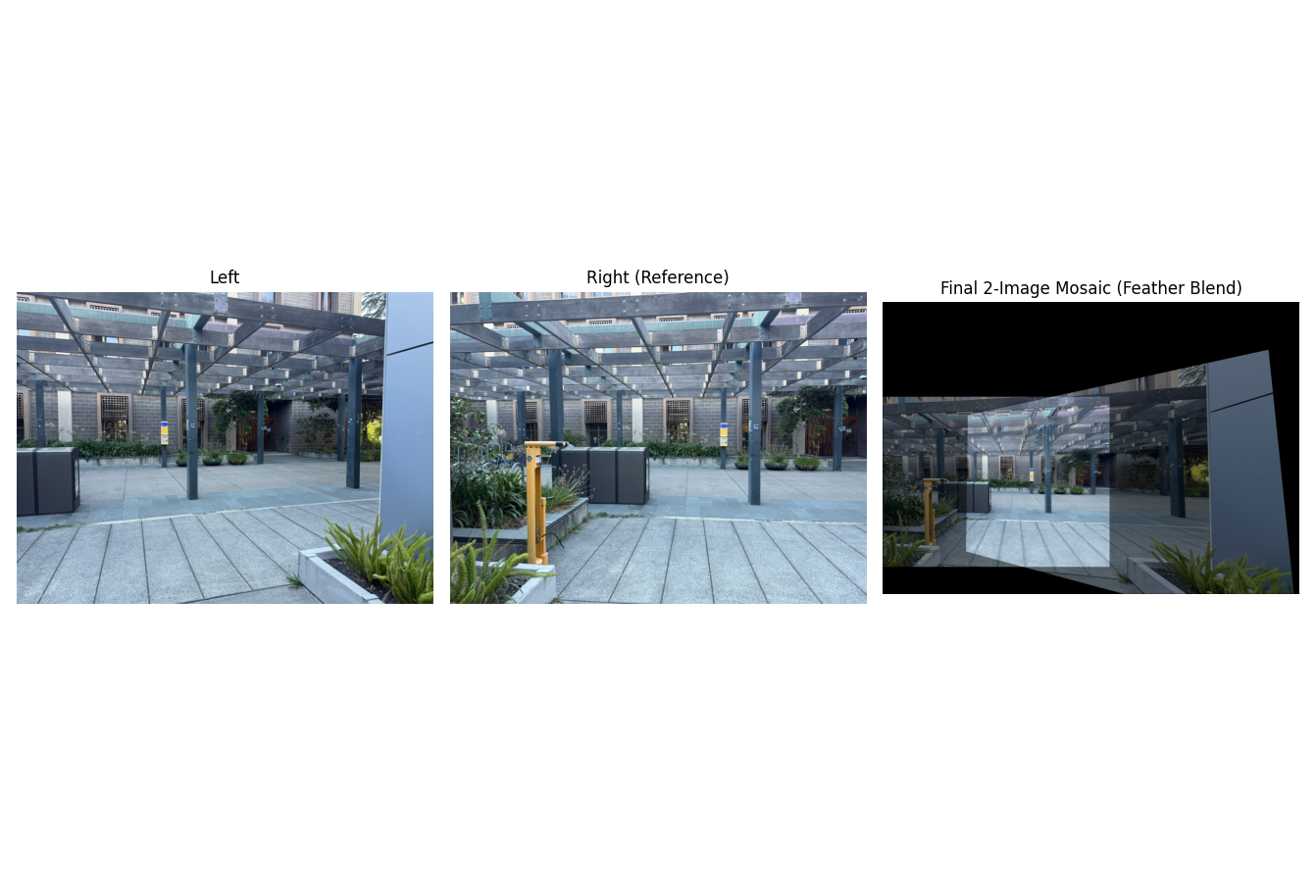
Extra: Scenic two-image mosaic

Notes on quality: feathering hides seams but can “ghost” high-frequency details when I can't hold a camera steady. A Laplacian-pyramid blend could further reduce that ghosting by separating low vs high frequencies during compositing.

Implementation Notes (brief)

• Global canvas is computed by warping all four corners of each image with its homography and taking the min/max over all.
• Everything is inverse-warped into this shared frame; I use bilinear sampling for smoother results.
• Alpha mask: center ≈ 1, edges fall to 0; final color is a normalized weighted sum.

What I Learned

Small correspondence errors swing homographies a lot—click care matters. Inverse warping made it straightforward to avoid holes, and feathering was a simple, surprisingly effective first pass at blending. The toughest part was data capture (keeping rotation-only and enough visual overlap).

Overview

The second part of the project was to fully automate the mosaicing pipeline. This involved implementing the algorithm described in the paper "Multi-Image Matching using Multi-Scale Oriented Patches" by Brown et al. The steps included detecting Harris corners, using Adaptive Non-Maximal Suppression (ANMS) to select the best ones, extracting feature descriptors for each point, matching features between images, and finally using RANSAC to robustly compute the homography and stitch the images.

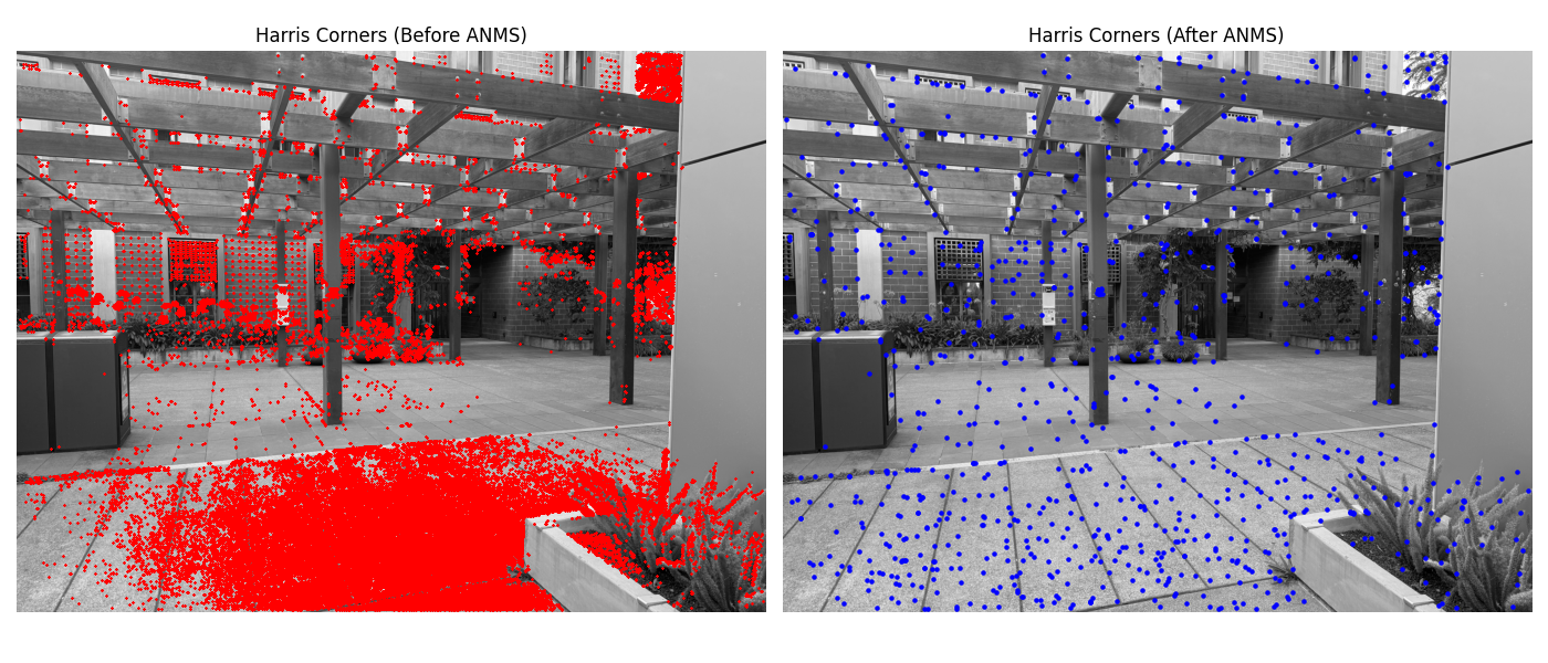
B.1 — Harris Corner Detection & ANMS

The first step is to identify interest points. I used the provided Harris corner detector to find thousands of potential feature points. However, this is too many and they are often poorly distributed. To fix this, I implemented Adaptive Non-Maximal Suppression (ANMS). For each point, ANMS finds the minimum radius to the nearest neighbor that has a significantly stronger corner strength. By selecting points with the largest suppression radii, we get a set of strong corners that are well-distributed across the image.

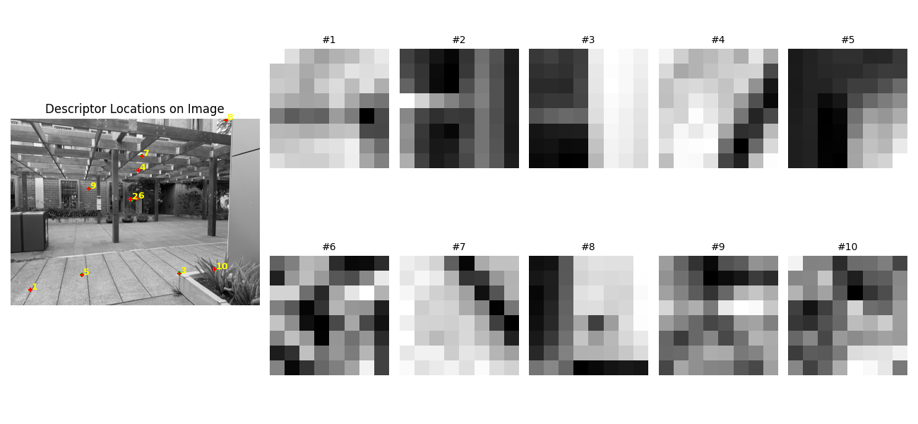
B.2 — Feature Descriptor Extraction

Once interest points are selected, we need a way to describe the local image patch around each one. Following the paper, I extracted a 40x40 pixel window around each corner, blurred it, and downsampled it to an 8x8 patch. This small, blurred patch serves as the feature descriptor. To make it robust to lighting changes, each 8x8 descriptor is bias/gain-normalized by subtracting its mean and dividing by its standard deviation.

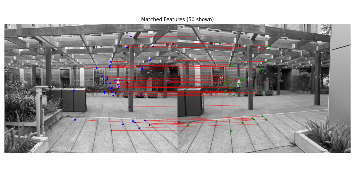
B.3 — Feature Matching

With descriptors for every feature point in two images, the next step is to find matching pairs. For each descriptor in the first image, I find its first and second nearest neighbors in the second image based on Euclidean distance. Following Lowe's ratio test, a match is considered valid only if the ratio of the distance to the first neighbor over the distance to the second neighbor is below a certain threshold (I used 0.5). This effectively rejects ambiguous matches where a point is almost equidistant to two different points in the other image.

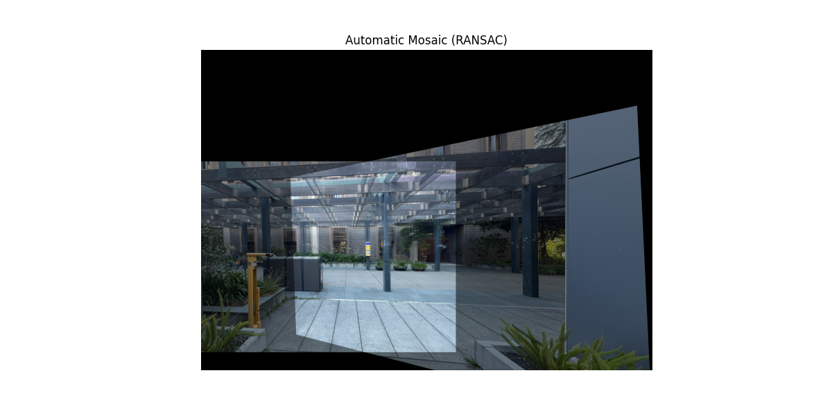
B.4 — RANSAC and Automatic Mosaics

The initial feature matches contain many incorrect outliers. To compute a robust homography, I implemented the RANSAC (Random Sample Consensus) algorithm. RANSAC iteratively selects a random sample of 4 point pairs, computes a candidate homography, and then counts how many other pairs ("inliers") agree with this model within a certain error tolerance. After many iterations, it chooses the homography that had the largest set of inliers and re-computes a final, more accurate homography using all of them. This process effectively ignores the outliers.

Below are three final mosaics created using this fully automatic pipeline. The results are compared with the manual mosaics from Part A.

Auto-Mosaic 1 — Breezeway

Part A: Manual Stitching

Part B: Automatic Stitching

Auto-Mosaic 2 — Scenic

Part A: Manual Stitching

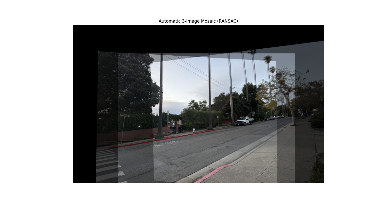
Part B: Automatic Stitching

Auto-Mosaic 3 — Whiteboard

Part A: Manual Stitching

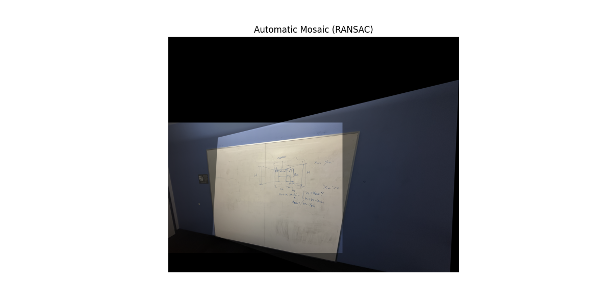
Part B: Automatic Stitching

What I Learned (Part B)

Automating the pipeline was a fantastic learning experience. The biggest takeaway was that RANSAC and this automated point selection is cool, but it also attains similar results to regular ginput; Finally, debugging the whole pipeline taught me the importance of coordinate system consistency (`(y,x)` vs. `(x,y)`) at every step.