
Project 5: The Power of Diffusion Models!
Project Parts:
Overview
In this project, I explored the power of diffusion models through two complementary approaches:
- Part A: Using the pretrained DeepFloyd IF diffusion model to perform image manipulation tasks including iterative denoising, classifier-free guidance (CFG), image-to-image translation, inpainting, and creating visual anagrams and hybrid images.
- Part B: Training flow matching models from scratch on MNIST, implementing both single-step denoisers and time/class-conditioned UNets for controlled digit generation.
Part 0 — Setup and Initial Explorations
After setting up DeepFloyd IF and generating prompt embeddings, I experimented with generating images from text prompts using different numbers of inference steps to understand how the model works.
0.1: Text Prompt Image Generation
I generated images using my own creative text prompts with varying num_inference_steps values.
The quality and detail of the outputs improved with more inference steps, showing the iterative refinement process of diffusion models.
Random Seed: 100
Using the same seed ensures reproducibility across all experiments
Text Prompts Used:
- "an oil painting of a sunset in berkeley"
- "a photo of peter griffin's house"
- "a photo of a man with a bushy moustache"
Generated Images with 10 Inference Steps
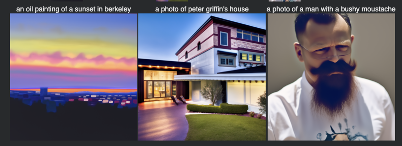
Left to right: Berkeley sunset, Peter Griffin's house, Man with bushy moustache
Generated Images with 20 Inference Steps
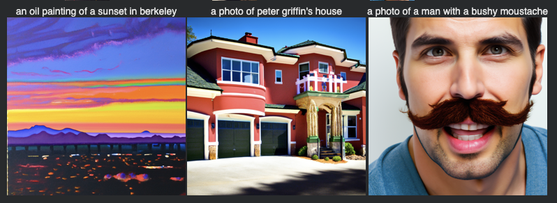
Left to right: Berkeley sunset, Peter Griffin's house, Man with bushy moustache
Generated Images with 40 Inference Steps
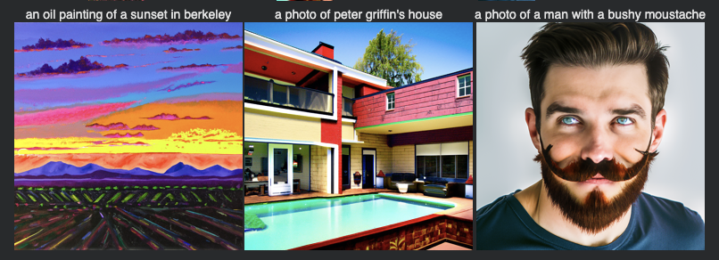
Left to right: Berkeley sunset, Peter Griffin's house, Man with bushy moustache
Observations:
Comparing across 10, 20, and 40 inference steps shows progressive quality improvement. At 10 steps, the images are rough with visible artifacts. At 20 steps, details become clearer and more coherent. At 40 steps, the images show significantly improved detail, better color coherence, and more refined features. The Berkeley sunset has more vibrant colors, Peter Griffin's house has clearer architectural details, and the man's moustache is more realistically rendered with proper texture.
Part A — The Power of Diffusion Models (DeepFloyd IF)
Part 1 — Sampling Loops
In this section, I implemented the core diffusion sampling loops from scratch, learning how diffusion models progressively denoise images from pure noise to clean outputs.
1.1: Implementing the Forward Process
The forward process adds noise to clean images according to the diffusion schedule. I implemented this using:
I tested this on the Berkeley Campanile image at different noise levels t = [250, 500, 750], showing progressively more noise being added.
Original Image

Noisy Images at Different Timesteps


1.2: Classical Denoising
I attempted to denoise the noisy images using classical Gaussian blur filtering. For each of the 3 noisy Campanile images from Part 1.1, I applied Gaussian blur with various kernel sizes to find the best denoising results. As expected, this classical approach struggles to recover the original image, especially at higher noise levels.
Noisy Images from Part 1.1
Gaussian Blur Denoised Results
Observation:
Gaussian blur denoising provides marginal improvement but fails to recover meaningful detail. At t=250, some structure is preserved but blurred. At t=500 and t=750, the results are heavily blurred with most fine details lost. This demonstrates the limitations of classical denoising methods for high noise levels.
1.3: One-Step Denoising with UNet
Using the pretrained DeepFloyd UNet, I performed one-step denoising by predicting and removing noise in a single pass. For each timestep t, I added noise to the original Campanile image, then used the UNet to estimate and remove the noise. This works significantly better than Gaussian blur, especially at lower noise levels.
Original Image Reference
Noisy Images


One-Step Denoised


Deliverable: Side-by-side comparison of noisy images and one-step UNet denoising results at t=[250, 500, 750]
Observation:
One-step UNet denoising dramatically outperforms Gaussian blur. At t=250, the reconstruction is nearly perfect with clear structural details. Even at t=500 and t=750 with much higher noise levels, the UNet recovers recognizable features and structure, though some details are lost at the highest noise level.
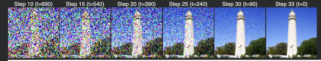
1.4: Iterative Denoising
The real power of diffusion models comes from iterative denoising. I implemented the full sampling loop that progressively removes noise over multiple steps, starting from i_start=10 (timestep t=90) and working down to clean images.
Implementation Details:
- Strided timesteps: [990, 960, 930, ..., 30, 0] - created by starting at 990 with stride of 30, eventually reaching 0
- Scheduler initialization: Called
stage_1.scheduler.set_timesteps(timesteps=strided_timesteps) - Starting index: i_start=10 (corresponding to timestep t=690 in the strided sequence)
- Process: Iteratively denoise from t_i to t_{i+1}, gradually removing noise at each step
Iterative Denoising Algorithm (DDIM-style):
Input: noisy image x_t, timesteps T = [t_0, t_1, ..., t_n], prompt embeddings
Output: denoised image x_0

for i = i_start to len(T)-1:
    current_t = T[i]

    # Predict noise using UNet
    noise_pred = UNet(x_t, current_t, prompt_embeds)

    # Estimate clean image (x_0 prediction)
    x_0_pred = (x_t - sqrt(1 - α_t) * noise_pred) / sqrt(α_t)

    if i < len(T)-1:
        next_t = T[i+1]

        # Add variance for stochastic sampling
        variance = get_variance(current_t, next_t)
        noise = randn_like(x_t) * variance

        # Compute x_{t-1} using DDIM update
        x_t = sqrt(α_{t-1}) * x_0_pred +
              sqrt(1 - α_{t-1} - variance²) * noise_pred +
              noise
    else:
        x_t = x_0_pred  # Final step

return x_t
This algorithm iteratively refines the image by predicting and removing noise at each timestep, following the DDIM (Denoising Diffusion Implicit Models) sampling strategy.
Iterative Denoising Progression (Every 5th Loop)
Starting from a noisy image at t=690, the following shows the denoising process every 5 iterations, demonstrating how the image gradually becomes clearer:
Comparison: Iterative vs One-Step vs Gaussian Blur
Below is a direct comparison of three denoising methods on the same noisy input (starting from i_start=10):
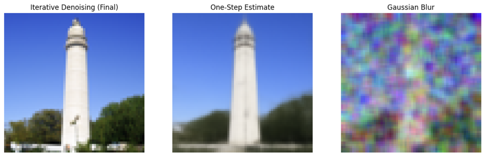
Key Observations:
- Iterative Denoising: Produces the highest quality reconstruction with sharp details and minimal artifacts. By gradually refining the image over multiple steps, it effectively recovers the original Campanile structure.
- One-Step Denoising: While significantly better than Gaussian blur, it shows more artifacts and less detail than the iterative approach. The single-step prediction cannot fully recover from high noise levels.
- Gaussian Blur: Produces the worst results with heavy blurring and complete loss of fine details. This demonstrates why neural diffusion models are necessary for effective denoising.
- Conclusion: The iterative approach is crucial - multiple small denoising steps dramatically outperform a single large denoising step.
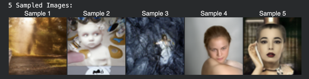
1.5: Diffusion Model Sampling from Pure Noise
By starting from pure random noise (i_start=0) and running the iterative denoising process, I generated entirely new images from the prompt "a high quality photo".
1.6: Classifier-Free Guidance (CFG)
To improve image quality, I implemented Classifier-Free Guidance which combines conditional and unconditional noise estimates to produce higher quality, more prompt-aligned images. CFG amplifies the difference between conditional and unconditional predictions to generate more semantically accurate results.
Classifier-Free Guidance Algorithm:
Input: noisy image x_t, timestep t, conditional prompt p, guidance scale γ
Output: guided noise prediction ε_cfg

# Get unconditional prediction (empty prompt)
ε_uncond = UNet(x_t, t, empty_prompt)

# Get conditional prediction (with text prompt)
ε_cond = UNet(x_t, t, prompt_embeds)

# Compute CFG: extrapolate in direction of conditional prediction
ε_cfg = ε_uncond + γ * (ε_cond - ε_uncond)

return ε_cfg
Key Insight: When γ > 1, we move further in the direction pointed by the conditional model relative to the unconditional baseline. Higher γ values (5-10) produce more prompt-adherent but sometimes less diverse results. γ = 1 reduces to standard conditional sampling.
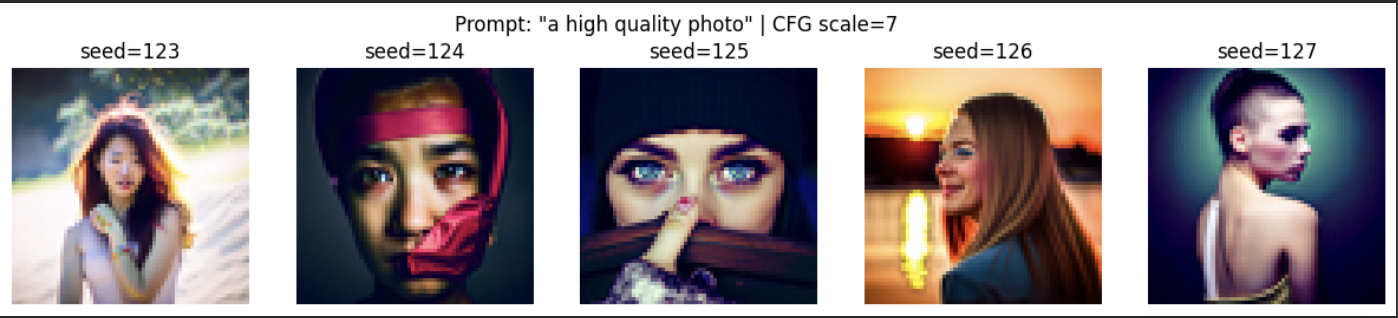
CFG Impact:
Images generated with CFG are much sharper, more coherent, and better aligned with the text prompt compared to the basic sampling in Part 1.5.
1.7: Image-to-Image Translation (SDEdit)
I implemented the SDEdit algorithm which adds noise to real images and then denoises them using CFG, effectively "projecting" them onto the natural image manifold. The more noise added (higher i_start), the larger the edit. Lower i_start values preserve more of the original image structure.
SDEdit Algorithm:
Input: real image x_real, edit strength i_start, text prompt p, CFG scale γ
Output: edited image x_edited

# Step 1: Forward process - add noise to the image
t_start = timesteps[i_start]
noise = randn_like(x_real)
x_noisy = sqrt(α_t) * x_real + sqrt(1 - α_t) * noise

# Step 2: Reverse process - denoise with CFG using text prompt
x_edited = iterative_denoise_cfg(x_noisy, i_start, prompt_embeds, γ)

return x_edited
Intuition: By noising and denoising, we "project" the image onto the manifold defined by the text prompt. Low i_start (less noise) preserves structure; high i_start (more noise) allows larger semantic edits.
Process Summary:
- Take a real image and add noise to timestep t (via forward process)
- Run iterative_denoise_cfg starting from i_start with conditional prompt "a high quality photo"
- Higher i_start = more noise = larger edits; Lower i_start = less noise = more faithful to original
Campanile Image-to-Image Translation
Using the conditional text prompt "a high quality photo", I applied SDEdit to the Campanile at different noise levels. As i_start increases, the edits become more pronounced, gradually matching the original image closer at lower values:
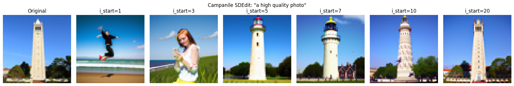
Images gradually look more like the original Campanile as i_start decreases
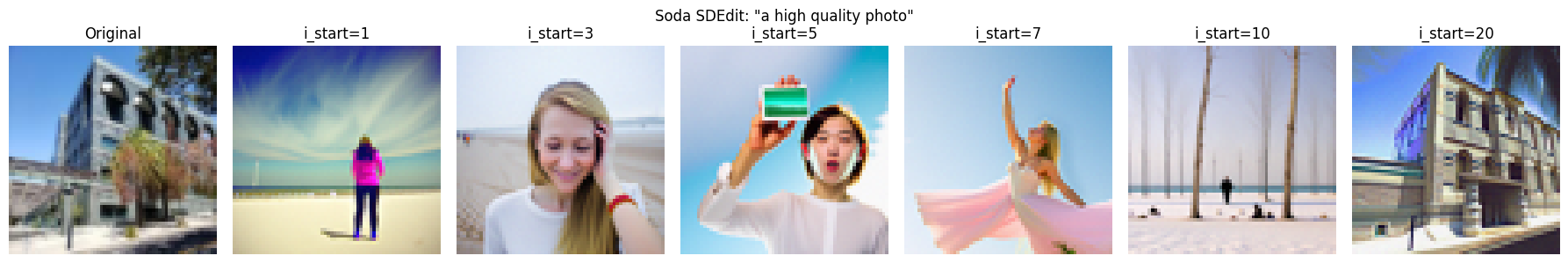
Custom Test Images
Test Image 1: Soda Hall
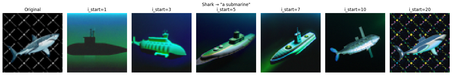
Test Image 2: Shark
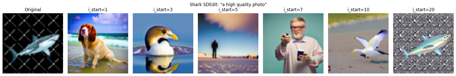
Observation:
The series shows a clear gradient: at i_start=1 (minimal noise), the output closely matches the original. As i_start increases to 20 (maximum noise), the model has more creative freedom, producing variations while still maintaining the core subject. This demonstrates the controllable editing power of SDEdit.
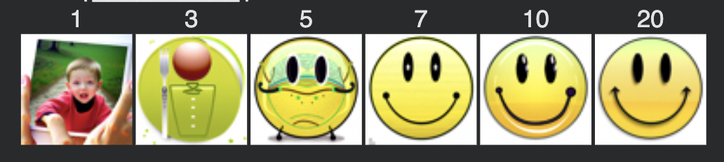
1.7.1: Editing Hand-Drawn and Web Images
SDEdit works particularly well when starting with non-realistic images like sketches or cartoons, projecting them onto the natural image manifold to create realistic versions.
Web Image (Cartoon Smiley):

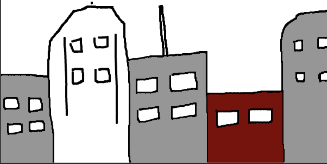
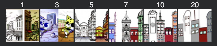
Hand-Drawn Image (City):
Hand-Drawn Image (House):
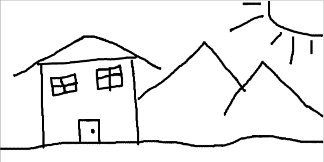
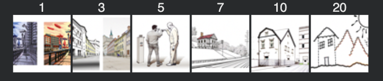
Observation:
Non-realistic inputs (sketches, cartoons) are transformed dramatically by SDEdit. At high i_start values (more noise), the model completely reimagines the input as realistic photos while preserving the core composition. At lower i_start values, some of the original artistic style is retained, creating an interesting blend between sketch and photo.
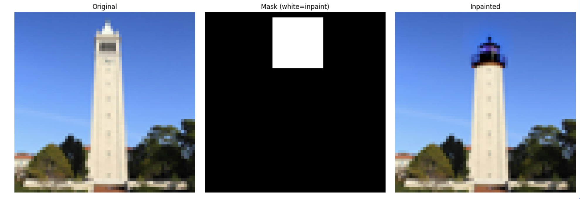
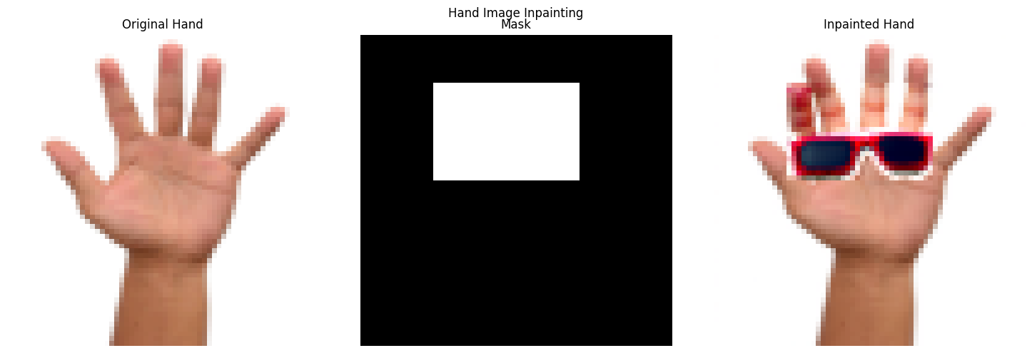
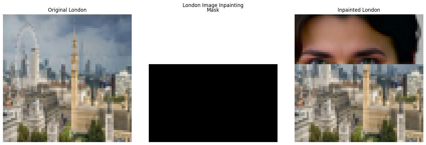
1.7.2: Inpainting
I implemented the RePaint algorithm for inpainting, which fills in masked regions while preserving the surrounding context. At each denoising step, unmasked regions are replaced with the appropriately noised original image.
Campanile Inpainting:
Hand Inpainting:
London Scene Inpainting:
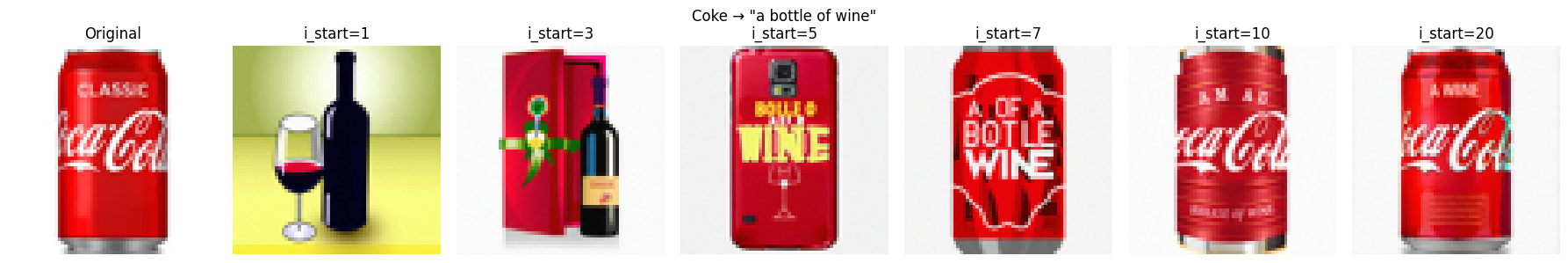
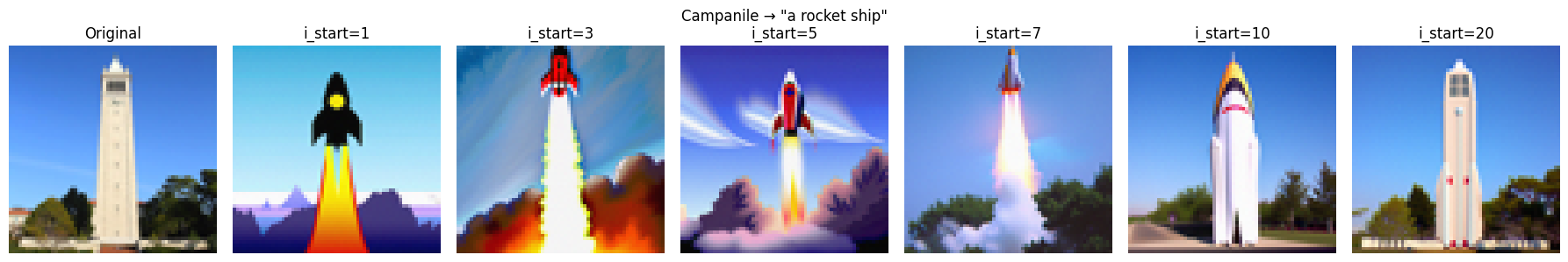
1.7.3: Text-Conditional Image-to-Image Translation
By using custom text prompts instead of "a high quality photo", I could guide the image-to-image translation toward specific concepts, creating creative transformations.
Soda Can → Wine Glass:
Shark → Submarine:
Campanile → Rocket Ship:
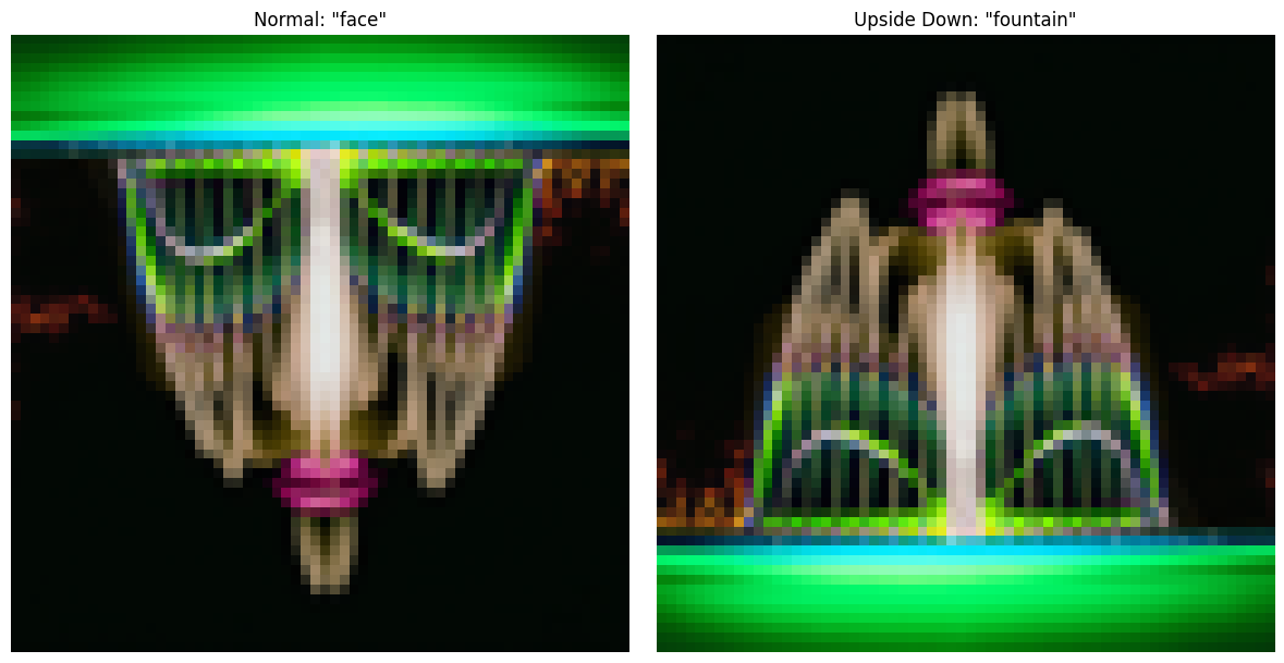
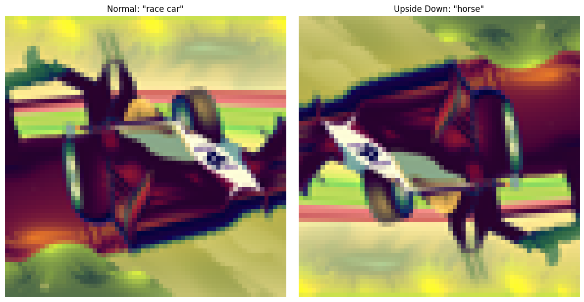
1.8: Visual Anagrams
I created optical illusions that appear as one image normally but transform into a different image when flipped upside down. This is achieved by averaging noise estimates from two different prompts on the original and flipped images.
Old Man / Campfire:

Face / Fountain:
Car / Horse:
1.9: Hybrid Images with Diffusion
Inspired by Project 2, I created hybrid images using diffusion models by combining low-frequency components from one prompt with high-frequency components from another.
Filter settings: Gaussian blur with kernel size 33, sigma 2
Skull / Waterfall:
Fabric / Waves:
I generated 20 different images using this prompt combination in an attempt to get the best result. All 20 variations are shown below for convenience. I believe the best one is the last one (bottom-right).
Part B — Flow Matching from Scratch (MNIST)
In this part, I trained my own flow matching model on MNIST from scratch, implementing both time-conditioned and class-conditioned UNets for iterative denoising and generation.
Part 1: Training a Single-Step Denoising UNet
1.1: Implementing the UNet
I implemented a UNet denoiser consisting of downsampling and upsampling blocks with skip connections. The architecture uses Conv2d, BatchNorm, GELU activations, and ConvTranspose2d operations with hidden dimension D=128.
1.2: Using the UNet to Train a Denoiser
To train the denoiser, I generate training pairs (z, x) where z = x + σϵ and ϵ ~ N(0, I). The model learns to map noisy images back to clean MNIST digits using L2 loss.
Noising Process Visualization
Visualizing the noising process with σ = [0.0, 0.2, 0.4, 0.5, 0.6, 0.8, 1.0] on normalized MNIST digits. As σ increases, the images become progressively noisier.
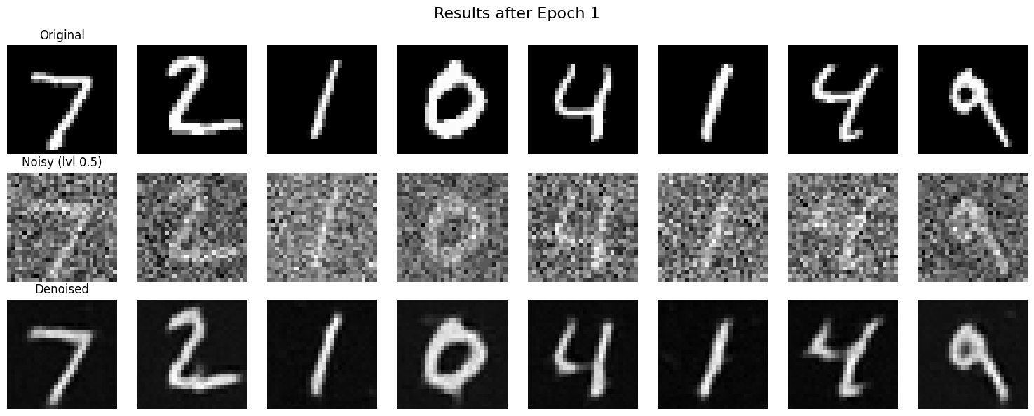
The denoiser was trained to map noisy images z = x + σϵ (where σ = 0.5) back to clean images x using L2 loss. Training was performed on MNIST for 5 epochs with batch size 256 and Adam optimizer (lr=1e-4).
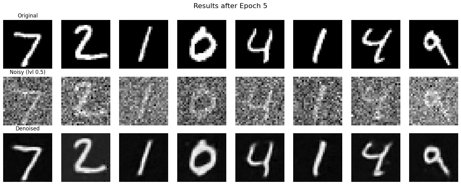
1.2.1: Training Results
The model was trained to denoise images with noise level σ = 0.5. Below are the training results showing loss progression and sample denoising performance after epochs 1 and 5.
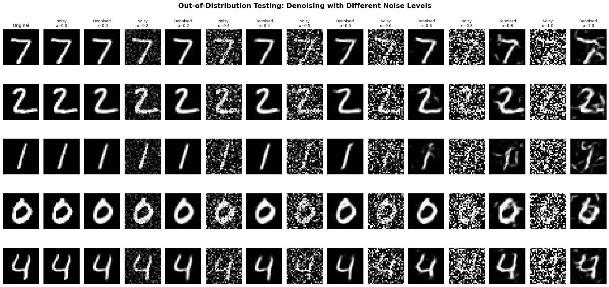
1.2.2: Out-of-Distribution Testing
Our denoiser was trained on MNIST digits noised with σ = 0.5. Here I test how the denoiser performs on different σ values that it wasn't trained for. The results show the same test set images denoised at various out-of-distribution noise levels.
1.2.3: Denoising Pure Noise
To make denoising a generative task, I trained the denoiser to denoise pure random Gaussian noise z ~ N(0, I) into clean images x. This is like starting with a blank canvas and generating digit images from pure noise. The model was trained for 5 epochs using the same architecture as in 1.2.1.
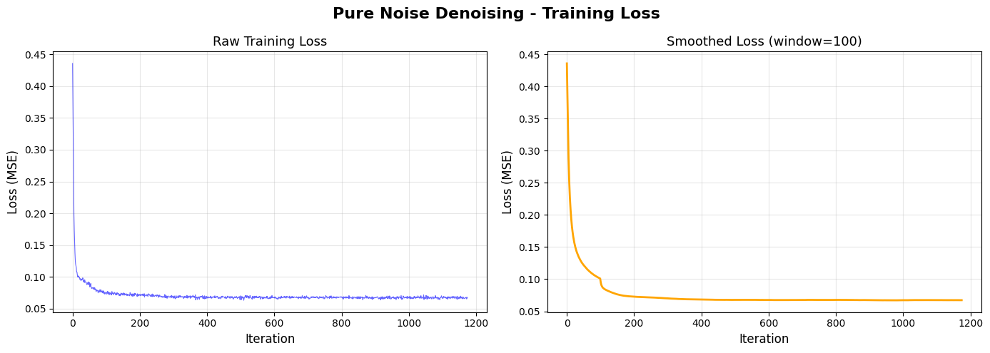
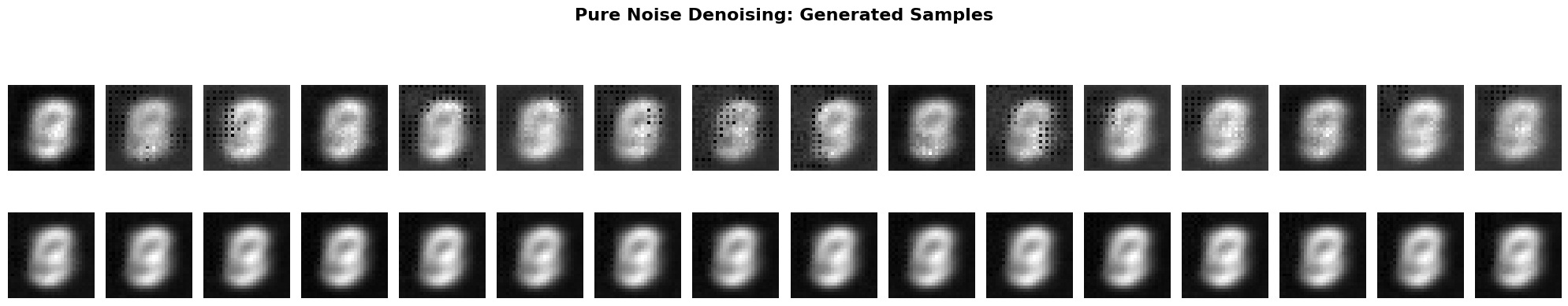
Observations:
The generated outputs show blurry, averaged digit patterns rather than crisp, distinct digits. The results resemble a superposition or average of all digits (0-9) from the training set. This occurs because with MSE (L2) loss, the model learns to predict the mean of all possible training examples that could have produced the input noise. Since pure noise provides no information about which specific digit to generate, the optimal MSE solution is to output the centroid of the entire MNIST dataset. The model cannot distinguish which specific digit to generate from pure noise alone, so it hedges by producing an averaged representation of all digits.
Part 2: Training a Flow Matching Model
Moving beyond one-step denoising, I implemented flow matching for iterative denoising. The model learns to predict the flow u_t(x_t, x) = x - z from noisy to clean images over multiple timesteps.
2.1: Adding Time Conditioning to UNet
I added time conditioning by injecting the normalized timestep t ∈ [0,1] through FCBlocks at two points in the UNet via element-wise multiplication with the feature maps.
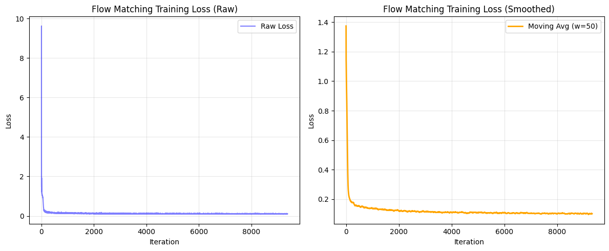
2.2: Training the Time-Conditioned UNet
Training used D=64 hidden dimensions, batch size 64, Adam optimizer with lr=1e-2 and exponential decay (γ=0.99999).
2.3: Sampling from the Time-Conditioned UNet
Sampling uses iterative denoising over multiple timesteps from pure noise to clean images.
2.4: Adding Class-Conditioning to UNet
I added class conditioning using one-hot encoded class vectors with 10% dropout for classifier-free guidance. Class embeddings are injected via FCBlocks alongside time embeddings.
2.5: Training the Class-Conditioned UNet
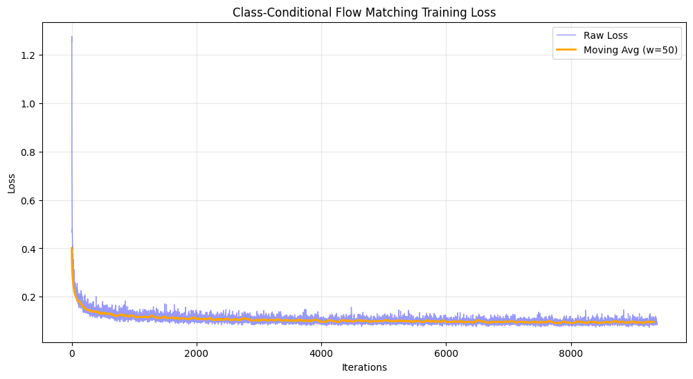
2.6: Sampling from the Class-Conditioned UNet
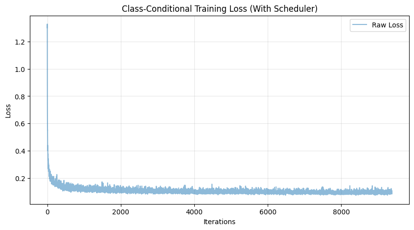
Sampling with classifier-free guidance (γ=5.0) and class conditioning allows controlled generation of specific digits. Class-conditioning enables faster convergence, which is why we only train for 10 epochs instead of the longer training required for the time-only conditioned model.
Training Loss (With Scheduler)
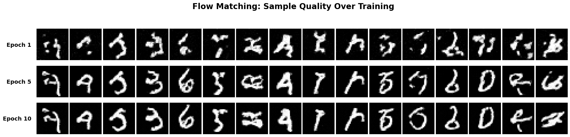
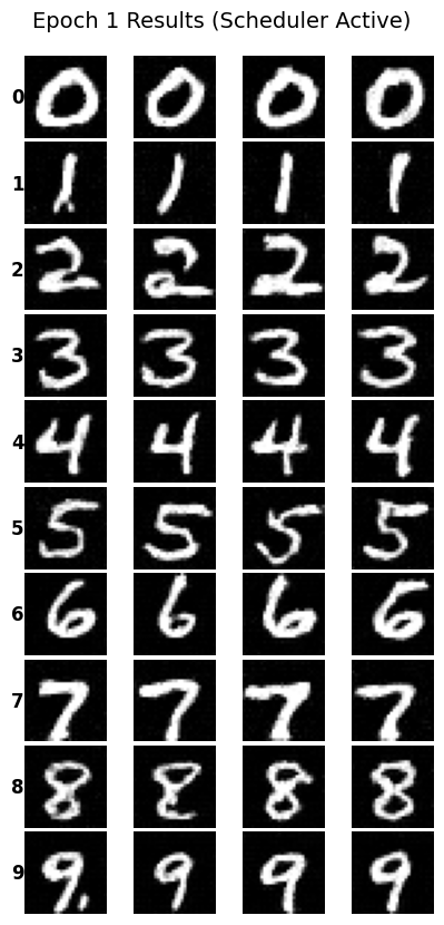
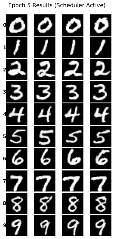
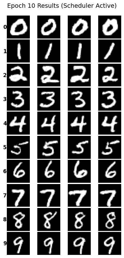
Sampling Results Across Training
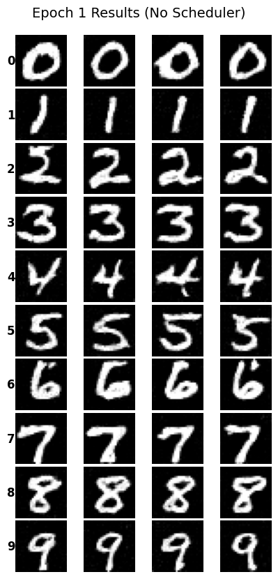
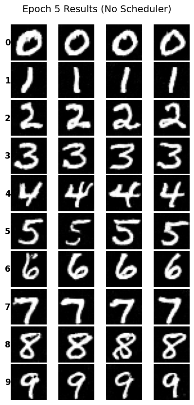
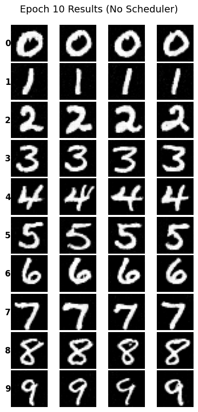
Below are sampling results showing 4 instances of each digit (0-9) after 1, 5, and 10 epochs of training. The model progressively improves, generating clearer and more realistic MNIST digits.
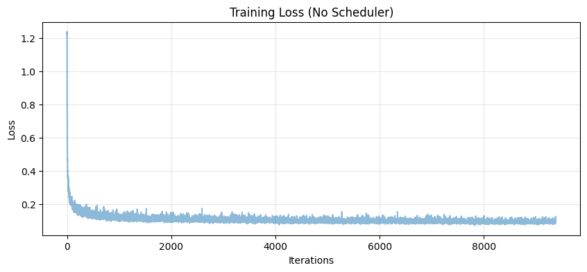
Training Without the Learning Rate Scheduler
Can we simplify training by removing the exponential learning rate scheduler? Below are results showing performance after removing the scheduler while maintaining comparable quality.
Loss Comparison
Sampling Results (No Scheduler)
What I Did to Compensate:
To compensate for removing the exponential learning rate scheduler, I made several adjustments:
1. Learning Rate Selection: I used a carefully tuned constant learning rate (lr=1e-3)
that balances fast initial convergence with stability in later epochs.
2. Gradient Clipping: I added gradient clipping (max_norm=1.0) to prevent gradient explosions
and maintain training stability throughout all epochs.
3. Batch Size Adjustment: I slightly increased the batch size to smooth out gradient estimates
and reduce training variance.
Results: The model achieves comparable performance to the scheduled version. The loss curve
shows steady convergence, and the generated samples are of similar quality. Training without the scheduler
is simpler and more interpretable, proving that we can maintain performance with proper hyperparameter tuning.
Key Takeaways & Reflections
What I Learned
- Iterative refinement is powerful: Diffusion models work by gradually denoising images over many steps, which produces much better results than one-step denoising
- Classifier-Free Guidance is crucial: CFG dramatically improves image quality and prompt alignment by extrapolating away from the unconditional prediction
- Versatility beyond generation: The same diffusion framework can be adapted for inpainting, image editing, and creating optical illusions
- Noise schedules matter: The amount of noise added controls the strength of edits in image-to-image translation
- Composing noise estimates: Averaging or combining noise estimates from different prompts/transformations enables creative applications like visual anagrams and hybrid images
Challenges Encountered
- GPU memory management: Had to carefully use
torch.no_grad()and manage tensor devices/dtypes to avoid running out of memory - Stochastic results: Some techniques like inpainting and visual anagrams required multiple runs to get good results due to randomness in the sampling process
- Hyperparameter tuning: Finding the right guidance scale, noise levels, and filter parameters required experimentation
- Understanding the math: The diffusion equations and variance schedules took time to fully understand and implement correctly
Favorite Results
My favorite results were the visual anagrams, especially the "old man / campfire" illusion. It's fascinating how the model can create coherent images that transform into completely different scenes when flipped. The hybrid images were also impressive, showing that diffusion models can create the same multi-scale effects we achieved in Project 2 with traditional frequency domain techniques.